Rents in San Francisco 2000-2018
In this case, we have a clean(ish) dataset with about 200K rows that corresponds to Craigslist listings for renting properties in the greater SF area. The data dictionary is as follows
| variable | class | description |
|---|---|---|
| post_id | character | Unique ID |
| date | double | date |
| year | double | year |
| nhood | character | neighborhood |
| city | character | city |
| county | character | county |
| price | double | price in USD |
| beds | double | n of beds |
| baths | double | n of baths |
| sqft | double | square feet of rental |
| room_in_apt | double | room in apartment |
| address | character | address |
| lat | double | latitude |
| lon | double | longitude |
| title | character | title of listing |
| descr | character | description |
| details | character | additional details |
The dataset was used in a recent tidyTuesday project.
# download directly off tidytuesdaygithub repo

rent <- readr::read_csv('https://raw.githubusercontent.com/rfordatascience/tidytuesday/master/data/2022/2022-07-05/rent.csv')
Cursory examination of data
The variable types are either character or double. On cursory glance, the variable types all tally. We sieved out all observations that had complete information to better check if the types correspond. From observation, the one variable type that seems not optimal is “date”, which is input as a “dbl”. This could (not should) be changed to the “date” type for heightened accuracy. The “chr” variables are all descriptors or names while the “dbl” variables are all numeric values; this checks out. The interesting thing to note is that the variable “address” is registered as “chr” type despite it being numeric; this is logical since the address is essentially a descriptor that serves as a categorical variable. The numeric aspect is not relevant for analysis. The top 5 variables that have the most missing values are “descr” (197542), “address” (196888), “lon” (196484), “lat” (193145) and “details” (192780).
glimpse(rent)## Rows: 200,796
## Columns: 17
## $ post_id <chr> "pre2013_134138", "pre2013_135669", "pre2013_127127", "pre…
## $ date <dbl> 20050111, 20050126, 20041017, 20120601, 20041021, 20060411…
## $ year <dbl> 2005, 2005, 2004, 2012, 2004, 2006, 2007, 2017, 2009, 2006…
## $ nhood <chr> "alameda", "alameda", "alameda", "alameda", "alameda", "al…
## $ city <chr> "alameda", "alameda", "alameda", "alameda", "alameda", "al…
## $ county <chr> "alameda", "alameda", "alameda", "alameda", "alameda", "al…
## $ price <dbl> 1250, 1295, 1100, 1425, 890, 825, 1500, 2925, 450, 1395, 1…
## $ beds <dbl> 2, 2, 2, 1, 1, 1, 1, 3, NA, 2, 2, 5, 4, 0, 4, 1, 3, 3, 1, …
## $ baths <dbl> 2, NA, NA, NA, NA, NA, 1, NA, 1, NA, NA, NA, 3, NA, NA, NA…
## $ sqft <dbl> NA, NA, NA, 735, NA, NA, NA, NA, NA, NA, NA, 2581, 1756, N…
## $ room_in_apt <dbl> 0, 0, 0, 0, 0, 0, 0, 0, 0, 0, 0, 0, 0, 0, 0, 0, 0, 0, 0, 0…
## $ address <chr> NA, NA, NA, NA, NA, NA, NA, NA, NA, NA, NA, NA, NA, NA, NA…
## $ lat <dbl> NA, NA, NA, NA, NA, NA, NA, NA, NA, NA, NA, NA, 37.5, NA, …
## $ lon <dbl> NA, NA, NA, NA, NA, NA, NA, NA, NA, NA, NA, NA, NA, NA, NA…
## $ title <chr> "$1250 / 2br - 2BR/2BA 1145 ALAMEDA DE LAS PULGAS", "$12…
## $ descr <chr> NA, NA, NA, NA, NA, NA, NA, NA, NA, NA, NA, NA, NA, NA, NA…
## $ details <chr> NA, NA, NA, NA, NA, NA, NA, NA, NA, NA, NA, NA, "<p class=…skimr::skim(rent)| Name | rent |
| Number of rows | 200796 |
| Number of columns | 17 |
| _______________________ | |
| Column type frequency: | |
| character | 8 |
| numeric | 9 |
| ________________________ | |
| Group variables | None |
Variable type: character
| skim_variable | n_missing | complete_rate | min | max | empty | n_unique | whitespace |
|---|---|---|---|---|---|---|---|
| post_id | 0 | 1.00 | 9 | 14 | 0 | 200796 | 0 |
| nhood | 0 | 1.00 | 4 | 43 | 0 | 167 | 0 |
| city | 0 | 1.00 | 5 | 19 | 0 | 104 | 0 |
| county | 1394 | 0.99 | 4 | 13 | 0 | 10 | 0 |
| address | 196888 | 0.02 | 1 | 38 | 0 | 2869 | 0 |
| title | 2517 | 0.99 | 2 | 298 | 0 | 184961 | 0 |
| descr | 197542 | 0.02 | 13 | 16975 | 0 | 3025 | 0 |
| details | 192780 | 0.04 | 4 | 595 | 0 | 7667 | 0 |
Variable type: numeric
| skim_variable | n_missing | complete_rate | mean | sd | p0 | p25 | p50 | p75 | p100 | hist |
|---|---|---|---|---|---|---|---|---|---|---|
| date | 0 | 1.00 | 2.01e+07 | 44694.07 | 2.00e+07 | 2.01e+07 | 2.01e+07 | 2.01e+07 | 2.02e+07 | ▁▇▁▆▃ |
| year | 0 | 1.00 | 2.01e+03 | 4.48 | 2.00e+03 | 2.00e+03 | 2.01e+03 | 2.01e+03 | 2.02e+03 | ▁▇▁▆▃ |
| price | 0 | 1.00 | 2.14e+03 | 1427.75 | 2.20e+02 | 1.30e+03 | 1.80e+03 | 2.50e+03 | 4.00e+04 | ▇▁▁▁▁ |
| beds | 6608 | 0.97 | 1.89e+00 | 1.08 | 0.00e+00 | 1.00e+00 | 2.00e+00 | 3.00e+00 | 1.20e+01 | ▇▂▁▁▁ |
| baths | 158121 | 0.21 | 1.68e+00 | 0.69 | 1.00e+00 | 1.00e+00 | 2.00e+00 | 2.00e+00 | 8.00e+00 | ▇▁▁▁▁ |
| sqft | 136117 | 0.32 | 1.20e+03 | 5000.22 | 8.00e+01 | 7.50e+02 | 1.00e+03 | 1.36e+03 | 9.00e+05 | ▇▁▁▁▁ |
| room_in_apt | 0 | 1.00 | 0.00e+00 | 0.04 | 0.00e+00 | 0.00e+00 | 0.00e+00 | 0.00e+00 | 1.00e+00 | ▇▁▁▁▁ |
| lat | 193145 | 0.04 | 3.77e+01 | 0.35 | 3.36e+01 | 3.74e+01 | 3.78e+01 | 3.78e+01 | 4.04e+01 | ▁▁▅▇▁ |
| lon | 196484 | 0.02 | -1.22e+02 | 0.78 | -1.23e+02 | -1.22e+02 | -1.22e+02 | -1.22e+02 | -7.42e+01 | ▇▁▁▁▁ |
rent_nomissing <- rent %>%
  drop_na()
head(rent_nomissing)
## # A tibble: 6 × 17
## post_id date year nhood city county price beds baths sqft room_…¹
## <chr> <dbl> <dbl> <chr> <chr> <chr> <dbl> <dbl> <dbl> <dbl> <dbl>
## 1 4710888130 20141012 2014 alameda alam… alame… 2250 2 1 1080 0
## 2 4988581576 20150421 2015 alameda alam… alame… 2650 2 1 950 0
## 3 4988561264 20150421 2015 alameda alam… alame… 1950 2 1 800 0
## 4 4855533017 20150120 2015 alameda alam… alame… 2650 2 1 950 0
## 5 4631188738 20140824 2014 alameda alam… alame… 3295 4 1 1716 0
## 6 4794051100 20141209 2014 alameda alam… alame… 1860 1 1 705 0
## # … with 6 more variables: address <chr>, lat <dbl>, lon <dbl>, title <chr>,
## # descr <chr>, details <chr>, and abbreviated variable name ¹room_in_apt
## # ℹ Use `colnames()` to see all variable names# Observe observations with complete information for better understanding of context
rent %>%
summarise_all(~sum(is.na(.))) %>%
gather() %>%
arrange(desc(value))## # A tibble: 17 × 2
## key value
## <chr> <int>
## 1 descr 197542
## 2 address 196888
## 3 lon 196484
## 4 lat 193145
## 5 details 192780
## 6 baths 158121
## 7 sqft 136117
## 8 beds 6608
## 9 title 2517
## 10 county 1394
## 11 post_id 0
## 12 date 0
## 13 year 0
## 14 nhood 0
## 15 city 0
## 16 price 0
## 17 room_in_apt 0# Check which variables have the most missing valuesPlot top 20 cities in terms of percent of total listings between 2000 and 2018
# Creating dataset with top 20 cities
top_cities <- rent %>%
  group_by(city) %>%
  summarize(count_city = n()) %>%
  arrange(desc(count_city)) %>%
  mutate(frequency = count_city / sum(count_city), frequency = parse_number(scales::percent(frequency)))%>%
  top_n(20)

# Plotting top 20 cities by % listings
ggplot(data = top_cities, mapping = aes(x = frequency, y = fct_reorder(city, frequency))) +
  geom_col() +
  labs(title = "Top 20 cities in terms of % of classifieds from 2000-2018", x = "Frequency (%)", y = "City") +
  theme(axis.title = element_text(size = 12), axis.text = element_text(size = 10))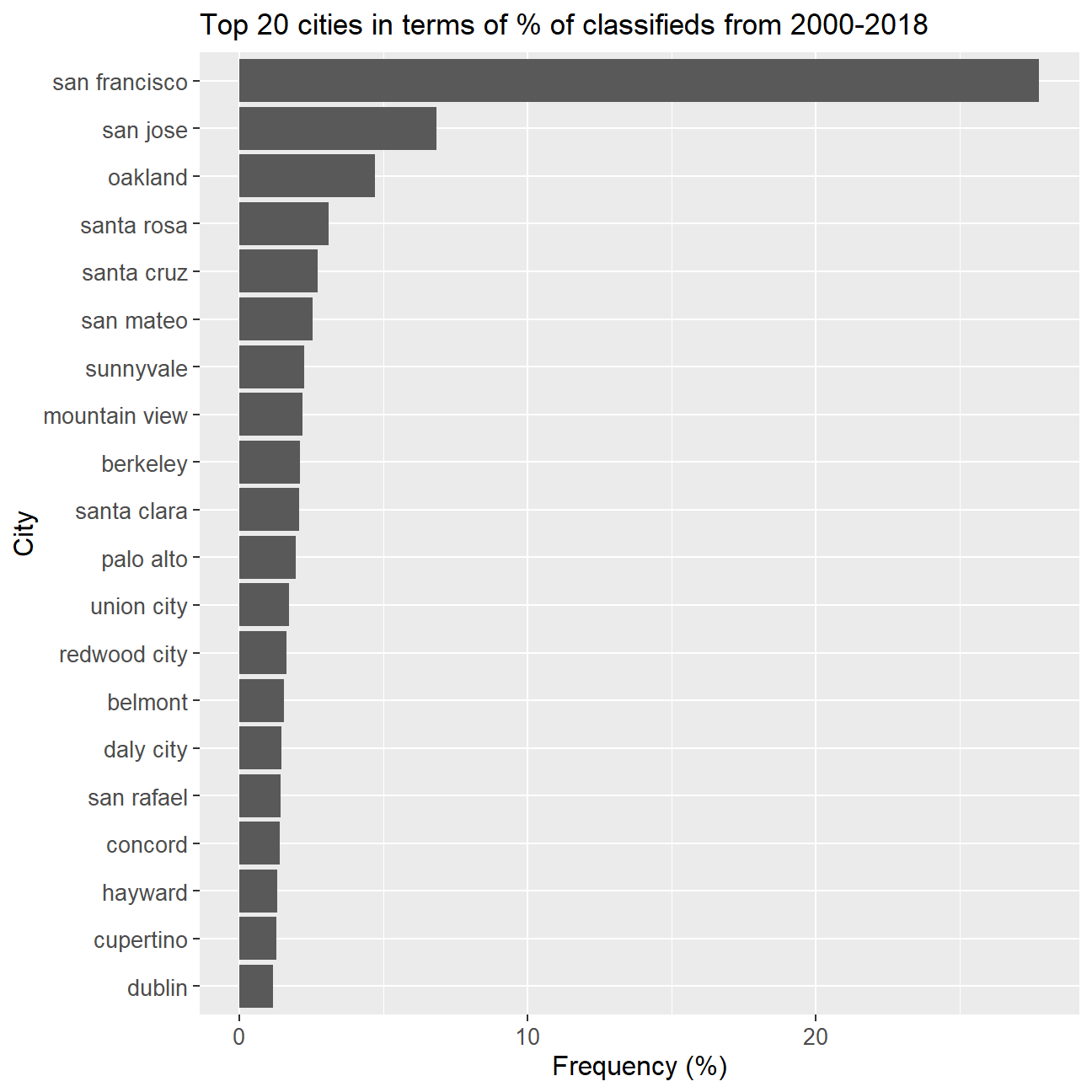
Plot the evolution of median prices of 0, 1, 2 and 3 bedroom-flats within San Francisco
# Created a table for the median price of flats with 3 or fewer bedrooms
median_price_beds <- rent %>%
  filter(beds <= 3 & city == "san francisco") %>%
  group_by(year, beds) %>%
  summarise(median_price = median(price))
median_price_beds
## # A tibble: 75 × 3
## # Groups: year [19]
## year beds median_price
## <dbl> <dbl> <dbl>
## 1 2000 0 1100
## 2 2000 1 2175
## 3 2000 2 2098.
## 4 2001 0 1250
## 5 2001 1 1725
## 6 2001 2 2250
## 7 2001 3 2995
## 8 2002 0 1125
## 9 2002 1 1532.
## 10 2002 2 1972.
## # … with 65 more rows
## # ℹ Use `print(n = ...)` to see more rows# Plotted the median price of flats with 3 or fewer bedrooms from 2000-2018
ggplot(data = median_price_beds, mapping = aes(year, median_price, colour = factor(beds))) +
facet_wrap(~ beds, ncol = 4) +
geom_line() +
scale_y_continuous(name = "Median price", breaks = seq(1000, 6000, 1000)) +
labs(title = str_wrap("Evolution of median prices in San Francisco for different number of beds", 60), x = "Year", y = "Median Price") +
theme(plot.title = element_text(size = 14, hjust = 0.5),
axis.title = element_text(size = 12),
axis.text = element_text(size = 10),
strip.text.x = element_text(size = 5)) +
theme(legend.key.size = unit(0.5, 'cm'), #change legend key size
legend.key.height = unit(0.5, 'cm'), #change legend key height
legend.key.width = unit(0.5, 'cm'), #change legend key width
legend.title = element_text(size=10), #change legend title font size
legend.text = element_text(size=8),
legend.position = "bottom") #change legend text font size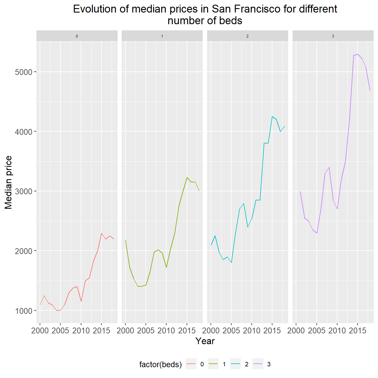
Plot the median price per city per year for flats in the top 12 cities (in terms of percent listings) from 2000 to 2018
# We used the description provided rather than what was shown in the plots; i.e. we took data from all number of bedrooms rather than just 1-bedroom like shown in the plots.

# Extract city names for top 12 cities into new dataframe (took a subset from an earlier section)
top_12 <- top_cities$city[1:12]

# Summarised median prices per city per year for the top 12 cities
median_top12_cities <- rent %>%
  filter(city %in% top_12) %>%
  group_by(city, year) %>%
  summarise(median_price = median(price))

# Plotted median prices per city per year for the top 12 cities from 2000-2018
ggplot(data = median_top12_cities, mapping = aes(year, median_price, colour = factor(city))) +
  facet_wrap(~ city, ncol = 4) +
  geom_line() +
  scale_y_continuous(name = "Median price", breaks = seq(1000, 6000, 1000)) +
  labs(title = "Median rental price for top 12 cities", x = "Year", y = "Median Price") +
  theme(plot.title = element_text(size = 14, hjust = 0.5),
        axis.title = element_text(size = 12),
        axis.text = element_text(size = 10),
        axis.text.x = element_text(angle = 90),
        strip.text.x = element_text(size = 10)) +
  theme(legend.key.size = unit(0.5, 'cm'), #change legend key size
        legend.key.height = unit(0.5, 'cm'), #change legend key height
        legend.key.width = unit(0.5, 'cm'), #change legend key width
        legend.title = element_text(size=10), #change legend title font size
        legend.text = element_text(size=8), #change legend text font size
        legend.position = "right")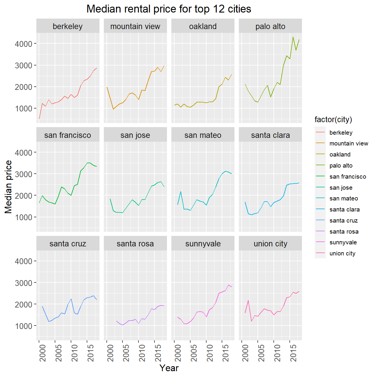
Inference and Analysis
We see that the median price of all flats with 3 or fewer bedrooms in San Francisco rose over the 15 years. It also seemed that the more bedrooms a flat had, the more severe the increase in price across years; 1-bed flats increased by about 100% of their original price after 15 years whereas 3-bed flats increased by 150%. We infer that a process of gentrification is at work here in the San Francisco region; wealthier individuals not only prefer, but also have the means to rent apartments with more luxurious amenities, e.g. more bedrooms. These individuals may engage in an auction process to out-bid their competitors to move into such apartments and thus prices rise more aggressively. One could also imagine that these apartments are within neighbourhoods with similar apartments; a process of gentrification then occurs since more wealthier individuals are attracted to these areas, thus fueling another cycle of competition and deepening the upward price spiral. While this cannot be seen from the plots, one could conduct spatial analysis/regression to test this narrative.
When the plots were faceted by cities, we see that the upward trend in prices still holds for all top 12 cities. However, the extent of overall increase in price within each city from 2000 to 2018 differs widely, with cities that experienced the highest price change suffering an almost 300% jump in price (Palo Alto) while other cities only saw a 100% increase in price. This suggests that some areas were more preferred than the others, perhaps due to better regional amenities maybe because they belonged to a more matured estate; the heightened demand for those areas caused an upward pressure on prices.
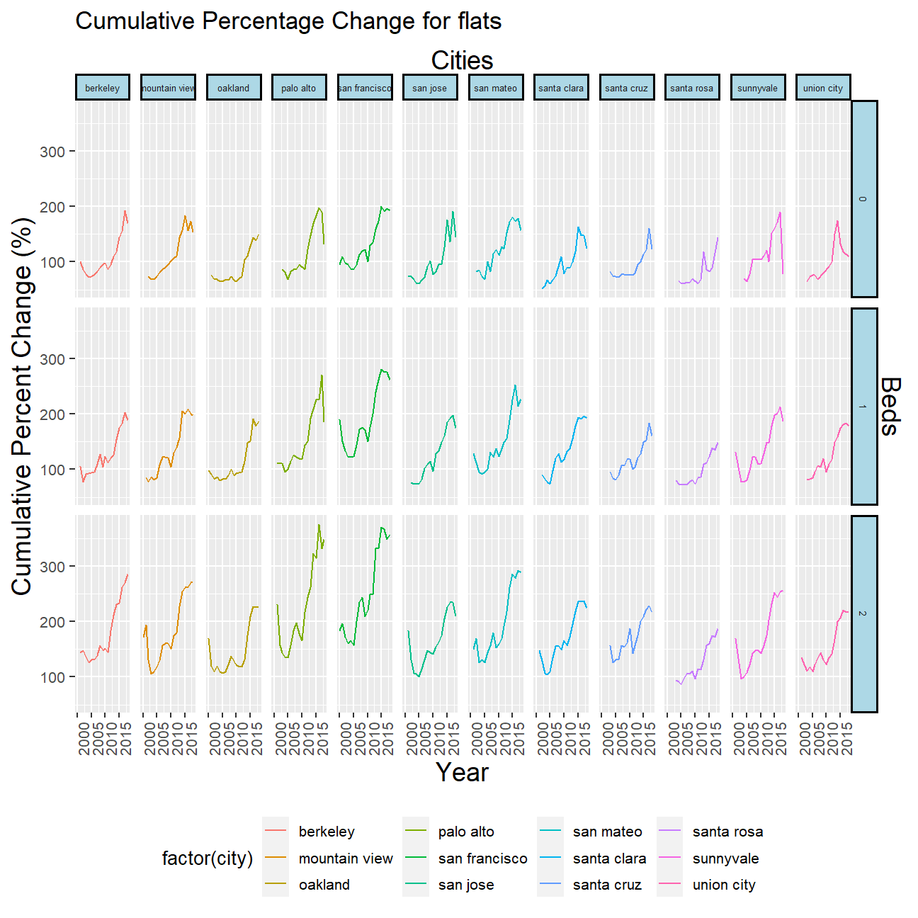
Plot cumulative percent change of median prices of 0, 1 and 2 bedroom flats for the top 12 cities in Bay Area
# Summarise popularity of cities in terms of percent of ads that appeared
# Find the top 12 cities (We reused code from the section above since they are linked)
top_12_cities <- rent %>%
  group_by(city) %>%
  summarize(count_city = n()) %>%
  arrange(desc(count_city)) %>%
  mutate(frequency = count_city / sum(count_city)) %>%
  top_n(12, frequency)

# View top 12 cities
top_12_cities
## # A tibble: 12 × 3
## city count_city frequency
## <chr> <int> <dbl>
## 1 san francisco 55730 0.278
## 2 san jose 13733 0.0684
## 3 oakland 9443 0.0470
## 4 santa rosa 6230 0.0310
## 5 santa cruz 5464 0.0272
## 6 san mateo 5127 0.0255
## 7 sunnyvale 4526 0.0225
## 8 mountain view 4414 0.0220
## 9 berkeley 4201 0.0209
## 10 santa clara 4171 0.0208
## 11 palo alto 3916 0.0195
## 12 union city 3451 0.0172# Based on the cumulative_percent_change code/formula that you sent us via Slack, we focused on the cumulative median price change
cumulative_percent_change <- rent %>%
filter(city %in% top_12_cities$city & beds <= 2) %>%
group_by(city, beds, year) %>%
summarise(median_price = median(price)) %>%
ungroup() %>%
mutate(pct_change = (median_price/lag(median_price))) %>%
mutate(pct_change = ifelse(is.na(pct_change), 1, pct_change)) %>%
mutate(percent_change = cumprod(pct_change), percent_change = parse_number(scales::percent(percent_change)))
# Plot cumulative percent median price change across time for each of the unique bed-city combination
ggplot(data = cumulative_percent_change, mapping = aes(year, percent_change, colour = factor(city))) +
facet_grid(vars(beds), vars(city)) +
geom_line() +
labs(title = "Cumulative Percentage Change for flats", x = "Year", y = "Cumulative Percent Change (%)", ) +
theme(axis.title = element_text(size = 14),
axis.text = element_text(size = 8),
axis.text.x = element_text(angle = 90),
strip.text = element_text(size = 5),
strip.background = element_rect(fill="lightblue", colour="black", size=1),
legend.key.size = unit(0.5, 'cm'), #change legend key size
legend.key.height = unit(0.5, 'cm'), #change legend key height
legend.key.width = unit(0.5, 'cm'), #change legend key width
legend.title = element_text(size=10), #change legend title font size
legend.text = element_text(size=8),
legend.position = "bottom") +
scale_x_continuous(sec.axis = sec_axis(~ . , name = "Cities", breaks = NULL, labels = NULL)) +
scale_y_continuous(sec.axis = sec_axis(~ . , name = "Beds", breaks = NULL, labels = NULL))