California Contributors plots
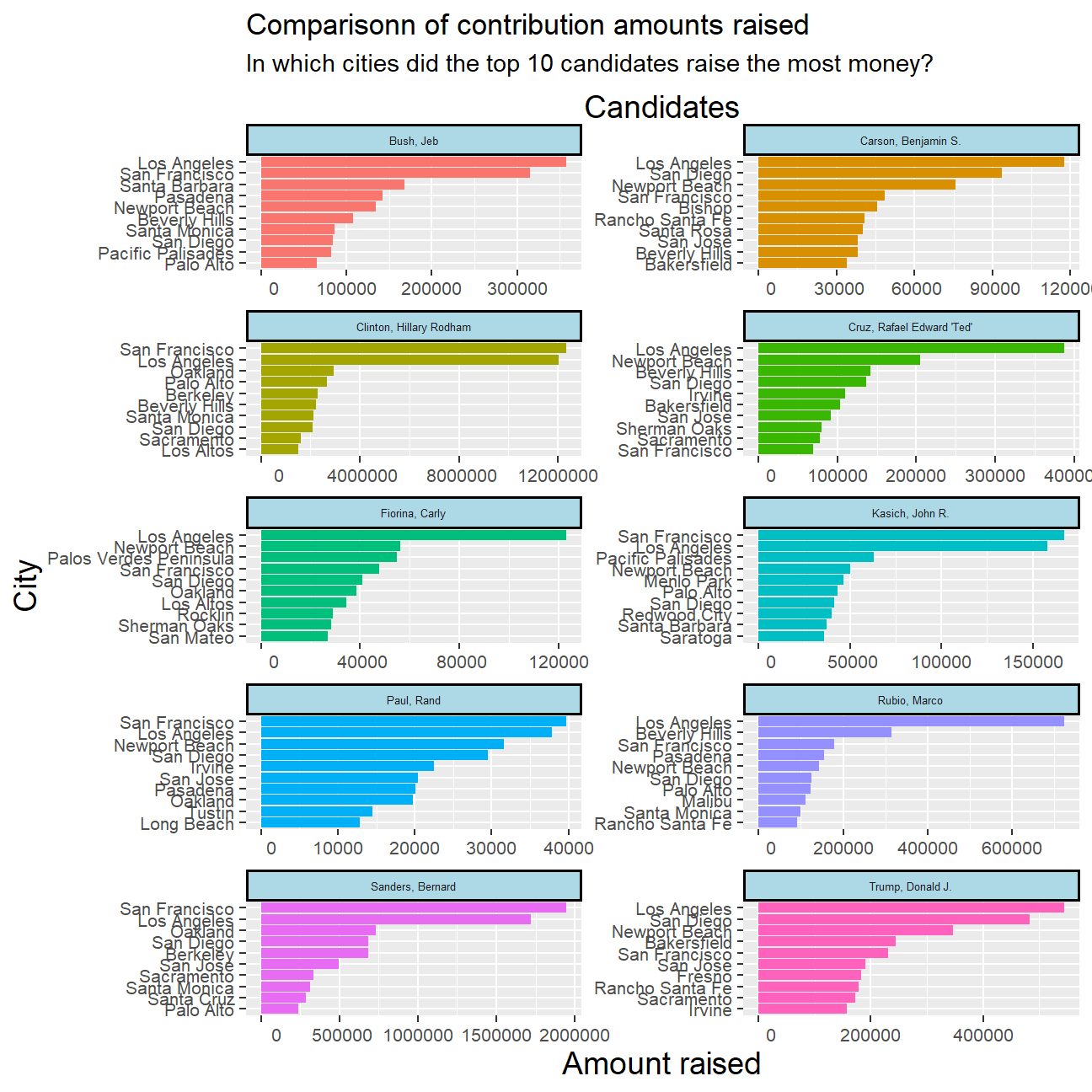
In this exercise, I plot the amounts raised in terms of political contributions by the top 10 candidates within their respective top 10 cities in California. The data used was from the year 2016.
Join dataframes
# Make sure you use vroom() as it is significantly faster than read.csv()
# Load datasets
CA_contributors_2016 <- vroom::vroom(here::here("data","CA_contributors_2016.csv"))

zipcodes <- read_csv(here::here("data", "zip_code_database.csv"))

# Glimpse datasets
glimpse(CA_contributors_2016)
## Rows: 1,292,843
## Columns: 4
## $ cand_nm <chr> "Clinton, Hillary Rodham", "Clinton, Hillary Rodham"…
## $ contb_receipt_amt <dbl> 50.0, 200.0, 5.0, 48.3, 40.0, 244.3, 35.0, 100.0, 25…
## $ zip <dbl> 94939, 93428, 92337, 95334, 93011, 95826, 90278, 902…
## $ contb_date <date> 2016-04-26, 2016-04-20, 2016-04-02, 2016-11-21, 201…glimpse(zipcodes)## Rows: 42,522
## Columns: 16
## $ zip <chr> "00501", "00544", "00601", "00602", "00603", "006…
## $ type <chr> "UNIQUE", "UNIQUE", "STANDARD", "STANDARD", "STAN…
## $ primary_city <chr> "Holtsville", "Holtsville", "Adjuntas", "Aguada",…
## $ acceptable_cities <chr> NA, NA, NA, NA, "Ramey", "Ramey", NA, NA, NA, NA,…
## $ unacceptable_cities <chr> "I R S Service Center", "Irs Service Center", "Co…
## $ state <chr> "NY", "NY", "PR", "PR", "PR", "PR", "PR", "PR", "…
## $ county <chr> "Suffolk County", "Suffolk County", "Adjuntas", N…
## $ timezone <chr> "America/New_York", "America/New_York", "America/…
## $ area_codes <dbl> 631, 631, 787939, 787, 787, NA, NA, 787939, 787, …
## $ latitude <dbl> 40.8, 40.8, 18.2, 18.4, 18.4, 18.4, 18.4, 18.2, 1…
## $ longitude <dbl> -73.0, -73.0, -66.7, -67.2, -67.2, -67.2, -67.2, …
## $ world_region <chr> NA, NA, NA, NA, NA, NA, NA, NA, NA, NA, NA, NA, N…
## $ country <chr> "US", "US", "US", "US", "US", "US", "US", "US", "…
## $ decommissioned <dbl> 0, 0, 0, 0, 0, 0, 0, 0, 0, 0, 0, 0, 0, 0, 0, 0, 0…
## $ estimated_population <dbl> 384, 0, 0, 0, 0, 0, 0, 0, 0, 0, 0, 0, 0, 0, 0, 0,…
## $ notes <chr> NA, NA, NA, NA, NA, NA, NA, NA, NA, "no NWS data,…# Join datasets (note that zip types are different across both datasets)
# Therefore we change them to be the same so that the datasets can be joined
CA_contributors_2016$zip<-as.character(CA_contributors_2016$zip)
df <- left_join(CA_contributors_2016, zipcodes, "zip")Create summary statistics
# Summarise total contributions raised by the top 10 candidates across every city
top_10_cand_overall <- df %>%
  group_by(cand_nm) %>%
  summarize(total = sum(contb_receipt_amt)) %>%
  arrange(desc(total)) %>%
  top_n(10)

# Create long form data to incude only the top 10 candidates
long_form_top10_cand_all_cities <- df %>%
  filter(cand_nm %in% top_10_cand_overall$cand_nm) %>%
  group_by(cand_nm, primary_city) %>%
  summarise(total_contrib = sum(contb_receipt_amt))

# From previous dataset, create a table for the top 10 candidates across the top 10 cities
# Incorporate the use of reorder_within to reorder within a group
top_10_cities_per_cand <- long_form_top10_cand_all_cities %>%
  group_by(cand_nm) %>%
  top_n(10, total_contrib) %>%
  ungroup() %>%
  mutate(cand_nm = as.factor(cand_nm),
         primary_city = tidytext::reorder_within(primary_city, total_contrib, cand_nm))
Plot political contributions raised by top 10 candidates in top 10 cities
# Plot faceted plots for each of the top 10 candidates across their respective top 10 cities
ggplot(top_10_cities_per_cand , aes(total_contrib, primary_city))+
  geom_col(aes(fill = cand_nm), show.legend = FALSE) +
  facet_wrap(~ cand_nm, ncol = 2, scales = "free") +
  tidytext::scale_y_reordered() +
  labs(title = "Comparisonn of contribution amounts raised", subtitle = "In which cities did the top 10 candidates raise the most money?", x = "Amount raised", y = "City") +
  theme(axis.title = element_text(size = 14),
          axis.text = element_text(size = 8),
          strip.text = element_text(size = 5),
          strip.background = element_rect(fill="lightblue", colour="black", size=1))+
  scale_x_continuous(labels = ~ format(.x, scientific = FALSE),
                     sec.axis = sec_axis(~ . , name = "Candidates", breaks = NULL, labels = NULL))