
Introduction and learning objectives
Load data
There are two sets of data, i) training data that has the actual prices ii) out of sample data that has the asking prices. Load both data sets.
#read in the data

# london_house_prices_2019_training<-read.csv("training_data_assignment_with_prices.csv")
# london_house_prices_2019_out_of_sample<-read.csv("test_data_assignment.csv")

london_house_prices_2019_training<- read_csv(here::here("data", "training_data_assignment_with_prices.csv"))
## Rows: 13998 Columns: 37
## ── Column specification ────────────────────────────────────────────────────────
## Delimiter: ","
## chr (18): postcode, property_type, whether_old_or_new, freehold_or_leasehol...
## dbl (18): ID, total_floor_area, number_habitable_rooms, co2_emissions_curre...
## date (1): date
##
## ℹ Use `spec()` to retrieve the full column specification for this data.
## ℹ Specify the column types or set `show_col_types = FALSE` to quiet this message.london_house_prices_2019_out_of_sample<-read_csv(here::here("data", "test_data_assignment.csv"))## Rows: 1999 Columns: 37
## ── Column specification ────────────────────────────────────────────────────────
## Delimiter: ","
## chr (12): property_type, whether_old_or_new, freehold_or_leasehold, town, po...
## dbl (18): ID, total_floor_area, number_habitable_rooms, co2_emissions_curren...
## lgl (7): date, postcode, address1, address2, address3, local_aut, county
##
## ℹ Use `spec()` to retrieve the full column specification for this data.
## ℹ Specify the column types or set `show_col_types = FALSE` to quiet this message.#fix data types in both data sets
#fix dates
london_house_prices_2019_training <- london_house_prices_2019_training %>% mutate(date=as.Date(date))
london_house_prices_2019_out_of_sample<-london_house_prices_2019_out_of_sample %>% mutate(date=as.Date(date))
#change characters to factors
london_house_prices_2019_training <- london_house_prices_2019_training %>% mutate_if(is.character,as.factor)
london_house_prices_2019_out_of_sample<-london_house_prices_2019_out_of_sample %>% mutate_if(is.character,as.factor)
#take a quick look at what's in the data
str(london_house_prices_2019_training)## tibble [13,998 × 37] (S3: tbl_df/tbl/data.frame)
## $ ID : num [1:13998] 2 3 4 5 7 8 9 10 11 12 ...
## $ date : Date[1:13998], format: "2019-11-01" "2019-08-08" ...
## $ postcode : Factor w/ 12635 levels "BR1 1AB","BR1 1LR",..: 10897 11027 11264 2031 11241 11066 421 9594 9444 873 ...
## $ property_type : Factor w/ 4 levels "D","F","S","T": 2 2 3 2 3 2 1 4 4 2 ...
## $ whether_old_or_new : Factor w/ 2 levels "N","Y": 1 1 1 1 1 1 1 1 1 1 ...
## $ freehold_or_leasehold : Factor w/ 2 levels "F","L": 2 2 1 2 1 2 1 1 1 2 ...
## $ address1 : Factor w/ 2825 levels "1","1 - 2","1 - 3",..: 2503 792 253 789 569 234 264 418 5 274 ...
## $ address2 : Factor w/ 434 levels "1","10","101",..: 372 NA NA NA NA NA NA NA NA NA ...
## $ address3 : Factor w/ 8543 levels "ABBERTON WALK",..: 6990 6821 3715 2492 4168 2879 3620 5251 6045 6892 ...
## $ town : Factor w/ 133 levels "ABBEY WOOD","ACTON",..: NA NA NA 78 NA NA NA NA NA NA ...
## $ local_aut : Factor w/ 69 levels "ASHFORD","BARKING",..: 36 46 24 36 24 46 65 36 36 17 ...
## $ county : Factor w/ 33 levels "BARKING AND DAGENHAM",..: 22 27 18 25 18 27 5 27 32 8 ...
## $ postcode_short : Factor w/ 247 levels "BR1","BR2","BR3",..: 190 194 198 28 198 194 4 169 167 8 ...
## $ current_energy_rating : Factor w/ 6 levels "B","C","D","E",..: 4 3 3 4 3 2 4 3 4 2 ...
## $ total_floor_area : num [1:13998] 30 50 100 39 88 101 136 148 186 65 ...
## $ number_habitable_rooms : num [1:13998] 2 2 5 2 4 4 6 6 6 3 ...
## $ co2_emissions_current : num [1:13998] 2.3 3 3.7 2.8 3.9 3.1 8.1 5.6 10 1.5 ...
## $ co2_emissions_potential : num [1:13998] 1.7 1.7 1.5 1.1 1.4 1.4 4.1 2 6.1 1.5 ...
## $ energy_consumption_current : num [1:13998] 463 313 212 374 251 175 339 216 308 128 ...
## $ energy_consumption_potential: num [1:13998] 344 175 82 144 90 77 168 75 186 128 ...
## $ windows_energy_eff : Factor w/ 5 levels "Average","Good",..: 1 1 1 5 1 1 1 1 5 1 ...
## $ tenure : Factor w/ 3 levels "owner-occupied",..: 1 2 1 2 1 1 1 2 1 1 ...
## $ latitude : num [1:13998] 51.5 51.5 51.5 51.6 51.5 ...
## $ longitude : num [1:13998] -0.1229 -0.2828 -0.4315 0.0423 -0.4293 ...
## $ population : num [1:13998] 34 75 83 211 73 51 25 91 60 97 ...
## $ altitude : num [1:13998] 8 9 25 11 21 11 95 7 7 106 ...
## $ london_zone : num [1:13998] 1 3 5 3 6 6 3 2 2 3 ...
## $ nearest_station : Factor w/ 592 levels "abbey road","abbey wood",..: 478 358 235 319 180 502 566 30 32 566 ...
## $ water_company : Factor w/ 5 levels "Affinity Water",..: 5 5 1 5 1 5 5 5 5 5 ...
## $ average_income : num [1:13998] 57200 61900 50600 45400 49000 56200 57200 65600 50400 52300 ...
## $ district : Factor w/ 33 levels "Barking and Dagenham",..: 22 27 18 26 18 27 5 27 32 8 ...
## $ price : num [1:13998] 360000 408500 499950 259999 395000 ...
## $ type_of_closest_station : Factor w/ 3 levels "light_rail","rail",..: 3 2 3 1 3 2 1 3 1 1 ...
## $ num_tube_lines : num [1:13998] 1 0 1 0 1 0 0 2 0 0 ...
## $ num_rail_lines : num [1:13998] 0 1 1 0 1 1 0 0 1 0 ...
## $ num_light_rail_lines : num [1:13998] 0 0 0 1 0 0 1 0 1 1 ...
## $ distance_to_station : num [1:13998] 0.528 0.77 0.853 0.29 1.073 ...str(london_house_prices_2019_out_of_sample)## tibble [1,999 × 37] (S3: tbl_df/tbl/data.frame)
## $ ID : num [1:1999] 14434 12562 8866 10721 1057 ...
## $ date : Date[1:1999], format: NA NA ...
## $ postcode : logi [1:1999] NA NA NA NA NA NA ...
## $ property_type : Factor w/ 4 levels "D","F","S","T": 1 2 2 3 4 3 2 3 2 4 ...
## $ whether_old_or_new : Factor w/ 2 levels "N","Y": 1 1 1 1 1 1 1 1 1 1 ...
## $ freehold_or_leasehold : Factor w/ 2 levels "F","L": 1 2 2 1 1 1 2 1 2 1 ...
## $ address1 : logi [1:1999] NA NA NA NA NA NA ...
## $ address2 : logi [1:1999] NA NA NA NA NA NA ...
## $ address3 : logi [1:1999] NA NA NA NA NA NA ...
## $ town : Factor w/ 54 levels "ACTON","ADDISCOMBE",..: NA NA NA NA NA NA NA NA NA NA ...
## $ local_aut : logi [1:1999] NA NA NA NA NA NA ...
## $ county : logi [1:1999] NA NA NA NA NA NA ...
## $ postcode_short : Factor w/ 221 levels "BR1","BR2","BR3",..: 82 50 37 52 214 150 159 115 175 126 ...
## $ current_energy_rating : Factor w/ 6 levels "B","C","D","E",..: 3 2 3 3 4 4 4 3 4 3 ...
## $ total_floor_area : num [1:1999] 150 59 58 74 97.3 ...
## $ number_habitable_rooms : num [1:1999] 6 2 2 5 5 5 5 4 2 5 ...
## $ co2_emissions_current : num [1:1999] 7.3 1.5 2.8 3.5 6.5 4.9 5.1 2.9 4.2 4.3 ...
## $ co2_emissions_potential : num [1:1999] 2.4 1.4 1.2 1.2 5.7 1.6 3 0.8 3.2 2.5 ...
## $ energy_consumption_current : num [1:1999] 274 142 253 256 303 309 240 224 458 253 ...
## $ energy_consumption_potential: num [1:1999] 89 136 110 80 266 101 140 58 357 143 ...
## $ windows_energy_eff : Factor w/ 5 levels "Average","Good",..: 1 1 1 1 1 1 3 1 3 1 ...
## $ tenure : Factor w/ 3 levels "owner-occupied",..: 1 1 1 1 1 1 1 1 1 1 ...
## $ latitude : num [1:1999] 51.6 51.6 51.5 51.6 51.5 ...
## $ longitude : num [1:1999] -0.129 -0.2966 -0.0328 -0.3744 -0.2576 ...
## $ population : num [1:1999] 87 79 23 73 100 24 22 49 65 98 ...
## $ altitude : num [1:1999] 63 38 17 39 8 46 26 16 14 18 ...
## $ london_zone : num [1:1999] 4 4 2 5 2 4 3 6 1 3 ...
## $ nearest_station : Factor w/ 494 levels "abbey wood","acton central",..: 16 454 181 302 431 142 20 434 122 212 ...
## $ water_company : Factor w/ 4 levels "Affinity Water",..: 4 1 4 1 4 4 4 2 4 4 ...
## $ average_income : num [1:1999] 61300 48900 46200 52200 60700 59600 64000 48100 56600 53500 ...
## $ district : Factor w/ 32 levels "Barking and Dagenham",..: 9 4 29 14 17 10 31 15 19 22 ...
## $ type_of_closest_station : Factor w/ 3 levels "light_rail","rail",..: 3 3 1 2 3 2 3 3 3 2 ...
## $ num_tube_lines : num [1:1999] 1 2 0 0 2 0 1 1 2 0 ...
## $ num_rail_lines : num [1:1999] 0 1 0 1 0 1 1 0 0 1 ...
## $ num_light_rail_lines : num [1:1999] 0 1 1 0 0 0 0 1 0 0 ...
## $ distance_to_station : num [1:1999] 0.839 0.104 0.914 0.766 0.449 ...
## $ asking_price : num [1:1999] 750000 229000 152000 379000 930000 350000 688000 386000 534000 459000 ...Set a seed for reproducibility
#initial split
library(rsample)
set.seed(100)
train_test_split <- initial_split(london_house_prices_2019_training, prop = 0.75) #training set contains 75% of the data
# Create the training dataset
train_data <- training(train_test_split)
test_data <- testing(train_test_split)
Visualize data
Visualize and examine the data
skimr::skim(train_data)| Name | train_data |
| Number of rows | 10498 |
| Number of columns | 37 |
| _______________________ | |
| Column type frequency: | |
| Date | 1 |
| factor | 18 |
| numeric | 18 |
| ________________________ | |
| Group variables | None |
Variable type: Date
| skim_variable | n_missing | complete_rate | min | max | median | n_unique |
|---|---|---|---|---|---|---|
| date | 0 | 1 | 2019-01-02 | 2019-12-29 | 2019-07-19 | 259 |
Variable type: factor
| skim_variable | n_missing | complete_rate | ordered | n_unique | top_counts |
|---|---|---|---|---|---|
| postcode | 0 | 1.00 | FALSE | 9688 | BR1: 4, E11: 4, E17: 4, IG8: 4 |
| property_type | 0 | 1.00 | FALSE | 4 | F: 4085, T: 3730, S: 2090, D: 593 |
| whether_old_or_new | 0 | 1.00 | FALSE | 2 | N: 10492, Y: 6 |
| freehold_or_leasehold | 0 | 1.00 | FALSE | 2 | F: 6316, L: 4182 |
| address1 | 0 | 1.00 | FALSE | 2308 | 3: 162, 7: 158, 12: 153, 4: 153 |
| address2 | 8061 | 0.23 | FALSE | 368 | FLA: 171, FLA: 167, FLA: 164, FLA: 121 |
| address3 | 0 | 1.00 | FALSE | 6968 | THE: 20, LON: 19, MAN: 18, GRE: 17 |
| town | 10018 | 0.05 | FALSE | 120 | CHE: 30, WAL: 30, STR: 24, CHI: 16 |
| local_aut | 0 | 1.00 | FALSE | 69 | LON: 5640, ROM: 299, BRO: 214, ILF: 179 |
| county | 0 | 1.00 | FALSE | 33 | BRO: 659, CRO: 535, WAN: 529, HAV: 504 |
| postcode_short | 0 | 1.00 | FALSE | 245 | CR0: 170, SW1: 145, E17: 141, SW1: 136 |
| current_energy_rating | 0 | 1.00 | FALSE | 6 | D: 5322, C: 2628, E: 1951, B: 278 |
| windows_energy_eff | 0 | 1.00 | FALSE | 5 | Ave: 5833, Goo: 2468, Ver: 1255, Poo: 939 |
| tenure | 0 | 1.00 | FALSE | 3 | own: 8431, ren: 1871, ren: 196 |
| nearest_station | 0 | 1.00 | FALSE | 586 | rom: 156, cha: 76, sid: 75, sur: 74 |
| water_company | 0 | 1.00 | FALSE | 5 | Tha: 7873, Aff: 1174, Ess: 861, SES: 587 |
| district | 0 | 1.00 | FALSE | 33 | Cro: 687, Bro: 641, Hav: 511, Bex: 449 |
| type_of_closest_station | 0 | 1.00 | FALSE | 3 | rai: 4870, tub: 3544, lig: 2084 |
Variable type: numeric
| skim_variable | n_missing | complete_rate | mean | sd | p0 | p25 | p50 | p75 | p100 | hist |
|---|---|---|---|---|---|---|---|---|---|---|
| ID | 0 | 1.00 | 7993.97 | 4613.41 | 2.00 | 4003.25 | 8044.50 | 11965.75 | 15996.00 | ▇▇▇▇▇ |
| total_floor_area | 0 | 1.00 | 92.31 | 44.70 | 21.00 | 64.00 | 83.00 | 108.00 | 480.00 | ▇▂▁▁▁ |
| number_habitable_rooms | 0 | 1.00 | 4.31 | 1.66 | 1.00 | 3.00 | 4.00 | 5.00 | 14.00 | ▆▇▁▁▁ |
| co2_emissions_current | 0 | 1.00 | 4.22 | 2.38 | 0.10 | 2.60 | 3.80 | 5.20 | 44.00 | ▇▁▁▁▁ |
| co2_emissions_potential | 0 | 1.00 | 2.21 | 1.44 | -0.30 | 1.30 | 1.80 | 2.70 | 19.00 | ▇▁▁▁▁ |
| energy_consumption_current | 0 | 1.00 | 262.22 | 93.63 | 12.00 | 201.00 | 249.00 | 306.75 | 1296.00 | ▇▅▁▁▁ |
| energy_consumption_potential | 0 | 1.00 | 141.31 | 77.71 | -34.00 | 89.00 | 122.00 | 167.00 | 1023.00 | ▇▂▁▁▁ |
| latitude | 0 | 1.00 | 51.49 | 0.08 | 51.30 | 51.43 | 51.49 | 51.56 | 51.68 | ▂▇▇▇▂ |
| longitude | 0 | 1.00 | -0.11 | 0.16 | -0.49 | -0.21 | -0.11 | 0.00 | 0.29 | ▂▅▇▅▂ |
| population | 56 | 0.99 | 83.86 | 43.97 | 1.00 | 52.00 | 79.00 | 109.00 | 510.00 | ▇▃▁▁▁ |
| altitude | 0 | 1.00 | 36.42 | 25.96 | 0.00 | 16.00 | 32.00 | 50.00 | 239.00 | ▇▃▁▁▁ |
| london_zone | 0 | 1.00 | 3.75 | 1.44 | 1.00 | 3.00 | 4.00 | 5.00 | 7.00 | ▇▇▇▆▅ |
| average_income | 0 | 1.00 | 55285.53 | 8437.85 | 36000.00 | 49300.00 | 54500.00 | 60600.00 | 85200.00 | ▃▇▆▂▁ |
| price | 0 | 1.00 | 590665.55 | 512740.51 | 77000.00 | 350000.00 | 460000.00 | 650000.00 | 10800000.00 | ▇▁▁▁▁ |
| num_tube_lines | 0 | 1.00 | 0.45 | 0.74 | 0.00 | 0.00 | 0.00 | 1.00 | 6.00 | ▇▁▁▁▁ |
| num_rail_lines | 0 | 1.00 | 0.58 | 0.51 | 0.00 | 0.00 | 1.00 | 1.00 | 2.00 | ▆▁▇▁▁ |
| num_light_rail_lines | 0 | 1.00 | 0.24 | 0.43 | 0.00 | 0.00 | 0.00 | 0.00 | 1.00 | ▇▁▁▁▂ |
| distance_to_station | 0 | 1.00 | 0.65 | 0.41 | 0.00 | 0.37 | 0.57 | 0.84 | 5.61 | ▇▁▁▁▁ |
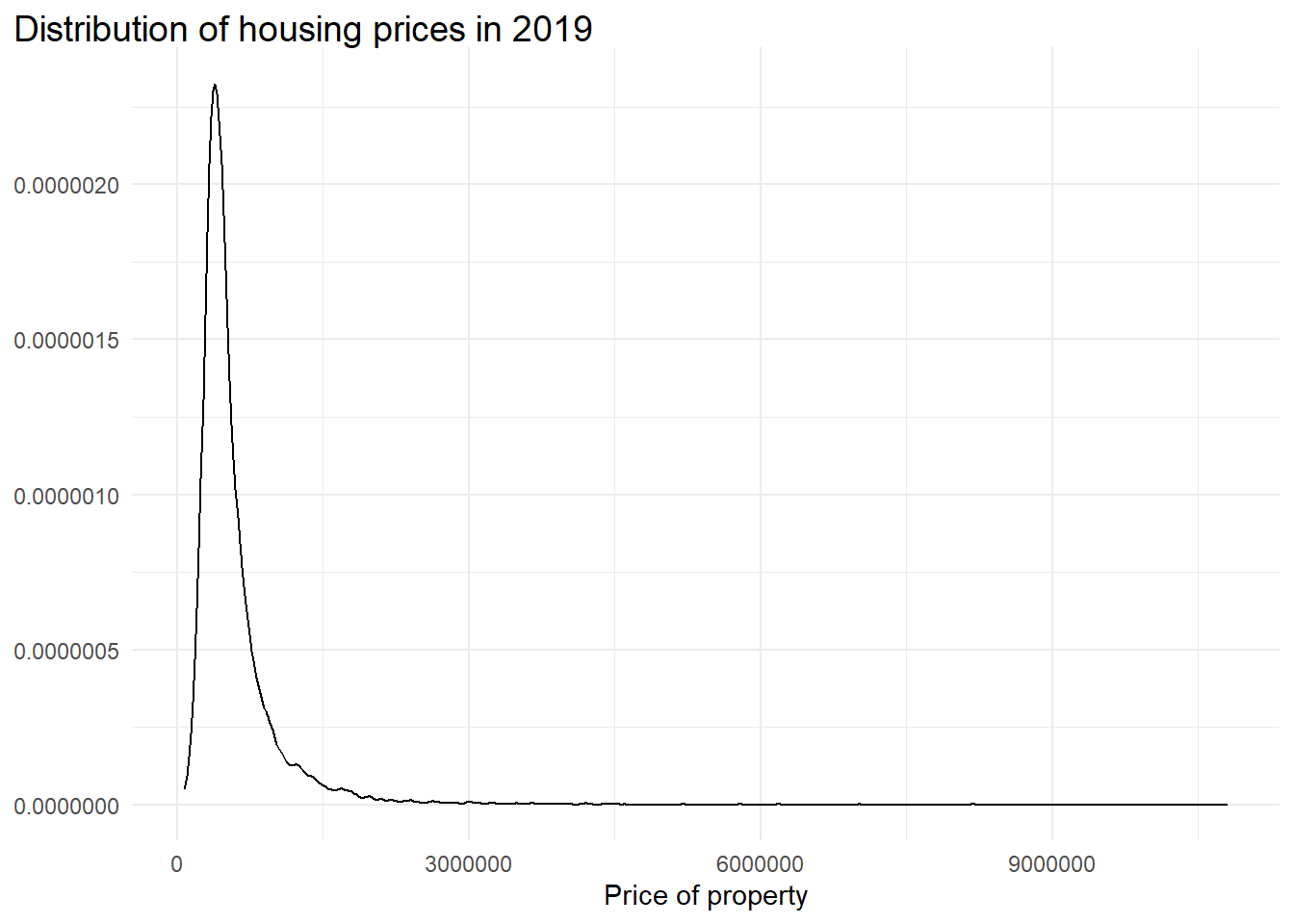
#plot distribution of property prices
ggplot(london_house_prices_2019_training, aes(x = price)) +
  geom_density() +
  theme_minimal() +
  labs(title = "Distribution of housing prices in 2019",
       x = "Price of property") +
  theme_minimal() +
  theme(plot.title.position = "plot",
        plot.title = element_textbox_simple(size = 14),
        axis.title.y = element_blank(),
        legend.position = "none",
        )
Let’s visualise the top 10 most expensive and bottom 10 least expensive districts in terms of average housing prices.
# Most expensive 10 districts
top10districts <- london_house_prices_2019_training %>%
  group_by(district) %>%
  summarise(average_price = mean(price)) %>%
  ungroup %>%
  arrange(desc(average_price)) %>%
  slice_max(average_price, n = 10) %>%
  ungroup()
top10districts
## # A tibble: 10 × 2
## district average_price
## <fct> <dbl>
## 1 Kensington and Chelsea 1859332.
## 2 Westminster 1278720.
## 3 Hammersmith and Fulham 1060149.
## 4 Camden 913301.
## 5 Richmond upon Thames 821685.
## 6 Islington 789380.
## 7 Wandsworth 786573.
## 8 City of London 680000
## 9 Barnet 669908.
## 10 Lambeth 656034.top_plot <- ggplot(top10districts, aes(x = average_price, y = fct_reorder(district, average_price))) +
geom_col(fill = "red") +
labs(
title = "<b>Most expensive 10 districts</b>",
x = "Average housing price") +
theme_minimal() +
theme(plot.title.position = "plot",
plot.title = element_textbox_simple(size = 14),
axis.title.y = element_blank(),
legend.position = "none",
strip.background =element_rect(fill="black"),
strip.text = element_text(colour = "white")
)
# Least expensive 10 districts
bot10districts <- london_house_prices_2019_training %>%
group_by(district) %>%
summarise(average_price = mean(price)) %>%
ungroup %>%
arrange(average_price) %>%
slice_min(average_price, n = 10) %>%
ungroup()
bot10districts## # A tibble: 10 × 2
## district average_price
## <fct> <dbl>
## 1 Barking and Dagenham 315135.
## 2 Newham 386354.
## 3 Bexley 389223.
## 4 Havering 397533.
## 5 Sutton 414071.
## 6 Hillingdon 447280.
## 7 Croydon 447403.
## 8 Waltham Forest 472370.
## 9 Enfield 476024.
## 10 Redbridge 479341.bot_plot <- ggplot(bot10districts, aes(x = average_price, y = fct_reorder(district, average_price))) +
geom_col(fill = "blue") +
labs(
title = "<b>Least expensive 10 districts</b>",
x = "Average housing price") +
theme_minimal() +
theme(plot.title.position = "plot",
plot.title = element_textbox_simple(size = 14),
axis.title.y = element_blank(),
legend.position = "none",
strip.background =element_rect(fill="black"),
strip.text = element_text(colour = "white")
)
#patchwork plot
top_plot + bot_plot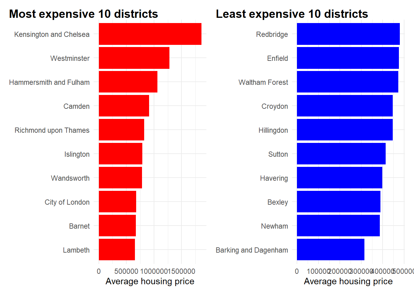
Estimate a correlation table between prices and other continuous variables
# correlation matrix
library("GGally")
london_house_prices_2019_training %>%
  select(-c(ID, london_zone, altitude, population, energy_consumption_current, energy_consumption_potential, co2_emissions_potential, total_floor_area)) %>% #keep Y variable last
  ggcorr(method = c("pairwise", "pearson"), layout.exp = 2,label_round=2, label = TRUE,label_size = 2,hjust = 1,nbreaks = 5,size = 2,angle = -20)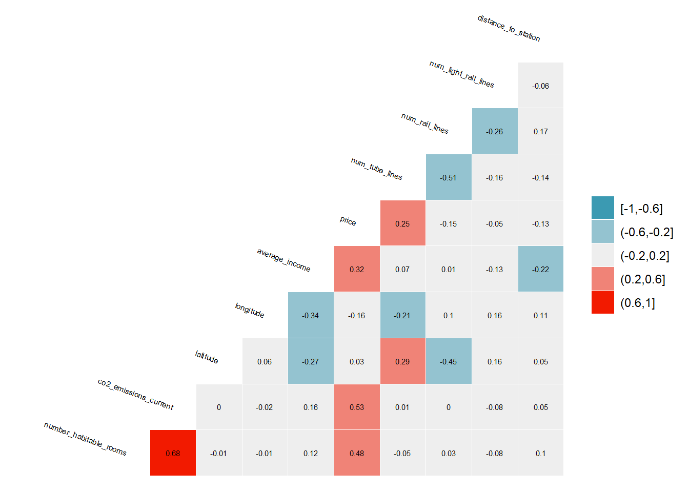
Model selection - An overview
The models that I will be testing will be:
Regression
- Linear regression (base)
Tree models
- Tree model (Base)
KNN model
LASSO Regression
Tree-based ensemble
Random Forest
Boosting
xgBoost
Let us define control parameters here.
#Define control variables
control <- trainControl (
    method = "cv",
    number = 10,
    verboseIter = FALSE) #by setting this to false the model will not report its progress after each estimation
Linear regression model (base)
To get started, I build a linear regression model below, choosing a subset of the features with no particular goal. These parameters and values form the basis as my benchmark model, with certain aspects that I define below.
I have chosen the number of folds for cross validation as 10.
I have added in additional features comprising:
Proxies for convenience through variables concerning public transportation - num_tube_lines, num_rail_lines, num_light_rail_lines These variables are important since it explains if the location of the property is close to an interchange. I would expect the prices of properties closer to interchanges to be more expensive since this creates an ability for residents to better commute to and from work with ease.
Proxies for affluence of neighbourhood - average_income, co2_emissions_current, districts
Condition/Type of house/property - number_habitable_rooms, windows_energy_eff, tenure
set.seed(100)
model1_lm<-train(
  price ~ distance_to_station + water_company + property_type + whether_old_or_new + freehold_or_leasehold + latitude + longitude + num_tube_lines + num_rail_lines + num_light_rail_lines + average_income + co2_emissions_current + number_habitable_rooms + district + windows_energy_eff + tenure,
  data = train_data,
  method = "lm",
  trControl = control
   )

# summary of the results
summary(model1_lm)
##
## Call:
## lm(formula = .outcome ~ ., data = dat)
##
## Residuals:
## Min 1Q Median 3Q Max
## -1654358 -124357 -5595 102272 7689396
##
## Coefficients:
## Estimate Std. Error t value
## (Intercept) -35903895.1977 9012033.9673 -3.984
## distance_to_station -17429.6497 9383.3137 -1.858
## `water_companyEssex & Suffolk Water` 65648.4282 42575.7340 1.542
## `water_companyLeep Utilities` 89313.0396 196663.1686 0.454
## `water_companySES Water` 50473.2984 34219.9169 1.475
## `water_companyThames Water` 151771.6977 22043.6976 6.885
## property_typeF -58552.8673 30845.2158 -1.898
## property_typeS -85555.3680 16288.8430 -5.252
## property_typeT -29520.7321 16444.0555 -1.795
## whether_old_or_newY 118688.8868 138654.6575 0.856
## freehold_or_leaseholdL -15005.6112 26164.5782 -0.574
## latitude 680940.6624 174741.9638 3.897
## longitude 589171.3898 109773.4861 5.367
## num_tube_lines 34619.0383 6505.8387 5.321
## num_rail_lines 8002.9677 9541.3327 0.839
## num_light_rail_lines 15792.2269 9766.5165 1.617
## average_income 9.6551 0.5016 19.249
## co2_emissions_current 64109.5597 2033.3681 31.529
## number_habitable_rooms 87762.4513 3204.0945 27.391
## districtBarnet 234836.5404 53987.6504 4.350
## districtBexley -93702.0684 49961.2779 -1.875
## districtBrent 346570.9672 57984.4826 5.977
## districtBromley 31150.5728 53382.7105 0.584
## districtCamden 490327.0824 52763.6522 9.293
## `districtCity of London` 437167.0967 158316.0616 2.761
## districtCroydon 120845.2237 55860.1822 2.163
## districtEaling 324384.0927 61886.7191 5.242
## districtEnfield -4188.6871 50967.4536 -0.082
## districtGreenwich 46067.2521 48987.6184 0.940
## districtHackney 309246.4759 49667.9964 6.226
## `districtHammersmith and Fulham` 655906.9933 59528.8789 11.018
## districtHaringey 188617.3726 52542.0836 3.590
## districtHarrow 265900.7284 66670.9941 3.988
## districtHavering -114495.3489 30627.5899 -3.738
## districtHillingdon 361153.0070 69291.7737 5.212
## districtHounslow 355116.2782 65217.2352 5.445
## districtIslington 438083.0869 52692.0432 8.314
## `districtKensington and Chelsea` 1355672.7518 56612.6146 23.946
## `districtKingston upon Thames` 287245.3052 63910.3910 4.495
## districtLambeth 297907.9710 53609.5904 5.557
## districtLewisham 110545.1677 50606.4472 2.184
## districtMerton 261587.3470 58643.1267 4.461
## districtNewham -5519.0071 49659.6740 -0.111
## districtRedbridge -76941.6128 37235.3528 -2.066
## `districtRichmond upon Thames` 406035.6635 64017.0071 6.343
## districtSouthwark 303305.7428 50489.3994 6.007
## districtSutton 249181.8886 62468.7138 3.989
## `districtTower Hamlets` 217271.5004 51025.0985 4.258
## `districtWaltham Forest` 38669.4205 47833.3189 0.808
## districtWandsworth 342524.4646 55393.8680 6.183
## districtWestminster 942367.6876 55735.6645 16.908
## windows_energy_effGood 60242.4460 8281.3348 7.274
## windows_energy_effPoor 51355.4998 12439.2507 4.129
## `windows_energy_effVery Good` -58129.9976 195379.5579 -0.298
## `windows_energy_effVery Poor` -9439.5870 11469.3623 -0.823
## `tenurerental (private)` -23297.9626 9071.1423 -2.568
## `tenurerental (social)` -14083.1964 24616.9164 -0.572
## Pr(>|t|)
## (Intercept) 0.000068226720079 ***
## distance_to_station 0.063266 .
## `water_companyEssex & Suffolk Water` 0.123123
## `water_companyLeep Utilities` 0.649736
## `water_companySES Water` 0.140251
## `water_companyThames Water` 0.000000000006109 ***
## property_typeF 0.057687 .
## property_typeS 0.000000153092734 ***
## property_typeT 0.072647 .
## whether_old_or_newY 0.392015
## freehold_or_leaseholdL 0.566313
## latitude 0.000098066609162 ***
## longitude 0.000000081701153 ***
## num_tube_lines 0.000000105204797 ***
## num_rail_lines 0.401619
## num_light_rail_lines 0.105914
## average_income < 0.0000000000000002 ***
## co2_emissions_current < 0.0000000000000002 ***
## number_habitable_rooms < 0.0000000000000002 ***
## districtBarnet 0.000013754326504 ***
## districtBexley 0.060753 .
## districtBrent 0.000000002347731 ***
## districtBromley 0.559547
## districtCamden < 0.0000000000000002 ***
## `districtCity of London` 0.005766 **
## districtCroydon 0.030537 *
## districtEaling 0.000000162317430 ***
## districtEnfield 0.934502
## districtGreenwich 0.347042
## districtHackney 0.000000000496029 ***
## `districtHammersmith and Fulham` < 0.0000000000000002 ***
## districtHaringey 0.000332 ***
## districtHarrow 0.000067015903052 ***
## districtHavering 0.000186 ***
## districtHillingdon 0.000000190320346 ***
## districtHounslow 0.000000052940886 ***
## districtIslington < 0.0000000000000002 ***
## `districtKensington and Chelsea` < 0.0000000000000002 ***
## `districtKingston upon Thames` 0.000007048401181 ***
## districtLambeth 0.000000028120195 ***
## districtLewisham 0.028954 *
## districtMerton 0.000008256009301 ***
## districtNewham 0.911510
## districtRedbridge 0.038819 *
## `districtRichmond upon Thames` 0.000000000235236 ***
## districtSouthwark 0.000000001949131 ***
## districtSutton 0.000066831450678 ***
## `districtTower Hamlets` 0.000020794824653 ***
## `districtWaltham Forest` 0.418867
## districtWandsworth 0.000000000650673 ***
## districtWestminster < 0.0000000000000002 ***
## windows_energy_effGood 0.000000000000373 ***
## windows_energy_effPoor 0.000036797065834 ***
## `windows_energy_effVery Good` 0.766073
## `windows_energy_effVery Poor` 0.410512
## `tenurerental (private)` 0.010232 *
## `tenurerental (social)` 0.567270
## ---
## Signif. codes: 0 '***' 0.001 '**' 0.01 '*' 0.05 '.' 0.1 ' ' 1
##
## Residual standard error: 337700 on 10441 degrees of freedom
## Multiple R-squared: 0.5686, Adjusted R-squared: 0.5662
## F-statistic: 245.7 on 56 and 10441 DF, p-value: < 0.00000000000000022# we can check variable importance as well
varImp(model1_lm)$importance %>%
as.data.frame() %>%
rownames_to_column() %>%
arrange(Overall) %>%
mutate(rowname = forcats::fct_inorder(rowname)) %>%
slice_max(Overall, n = 20) %>%
ggplot()+
geom_col(aes(x = rowname, y = Overall)) +
labs(y = "Importance", x = "") +
coord_flip() +
theme_bw()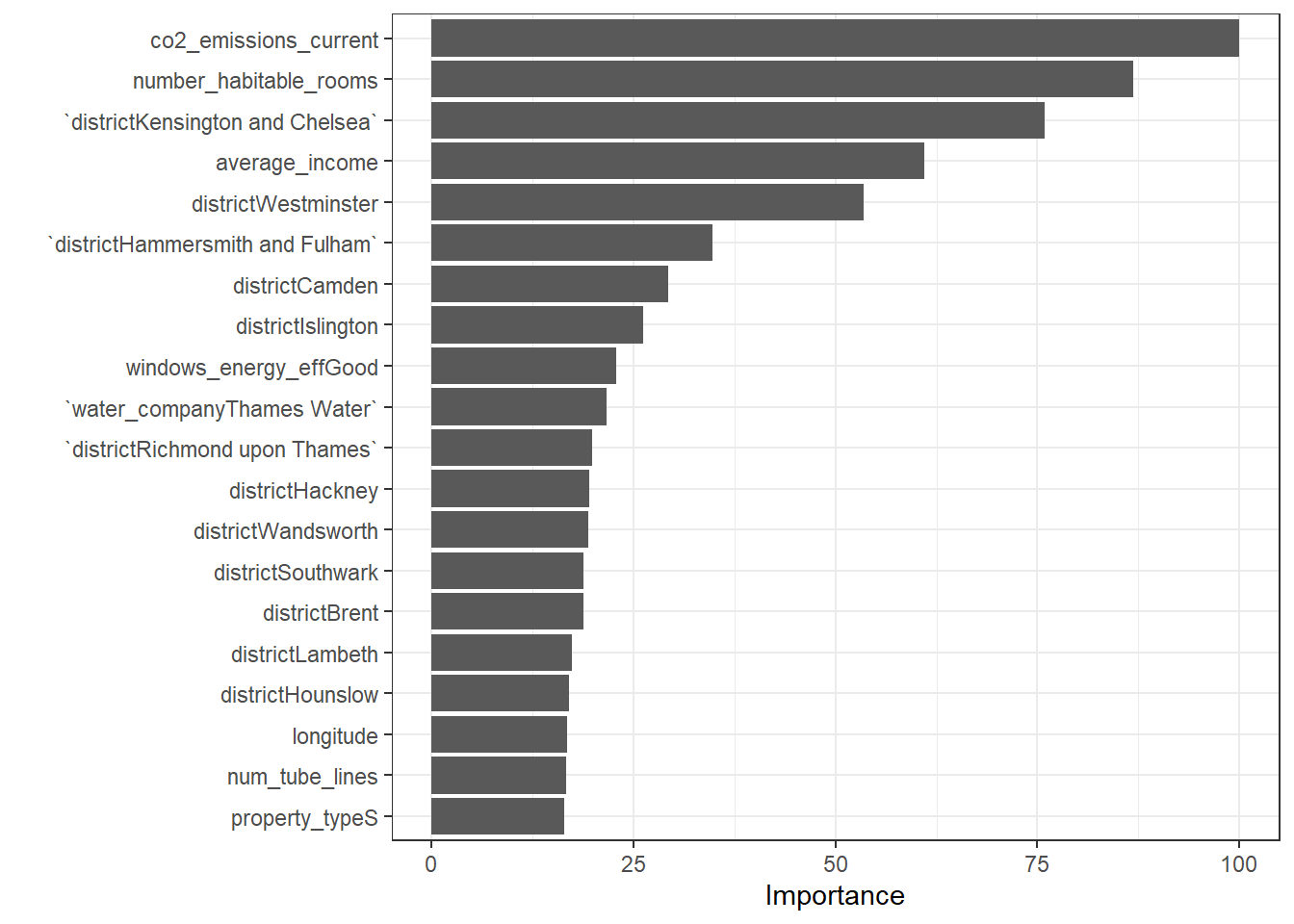
Predict the values in testing and out of sample data
Below I use the predict function to test the performance of the model in testing data and summarize the performance of the linear regression model
# predict testing values and RMSE
predictions <- predict(model1_lm,test_data)

lr_results<-data.frame(RMSE = RMSE(predictions, test_data$price),
                       Rsquare = R2(predictions, test_data$price))

lr_results
## RMSE Rsquare
## 1 333122.5 0.6187907Tree model (base) Model
Next I fit a tree model with some new variables introduced. This will be my base tree model for reference.
set.seed(100)
base_tree <- train(
  price ~ distance_to_station + water_company + property_type + whether_old_or_new + freehold_or_leasehold + latitude + longitude + num_tube_lines + num_rail_lines + num_light_rail_lines + average_income + co2_emissions_current + number_habitable_rooms + district + windows_energy_eff + tenure,
  data = train_data,
  method = "rpart",
  trControl = control,
  tuneLength=10
    )
## Warning in nominalTrainWorkflow(x = x, y = y, wts = weights, info = trainInfo,
## : There were missing values in resampled performance measures.#view tree performance
base_tree$results## cp RMSE Rsquared MAE RMSESD RsquaredSD MAESD
## 1 0.01116344 366490.8 0.4796808 208373.3 36052.49 0.09888230 8540.183
## 2 0.01224143 371350.6 0.4656442 211301.9 34143.11 0.10102365 7310.195
## 3 0.01468396 375630.6 0.4548960 214464.4 33599.60 0.10389302 7807.762
## 4 0.02024850 380978.2 0.4382873 219304.4 31773.34 0.10780441 6969.250
## 5 0.02755995 397833.2 0.3959637 223756.8 38869.20 0.08315648 8270.221
## 6 0.05429934 423868.5 0.3124573 237451.1 58281.24 0.08105167 13051.678
## 7 0.05492236 423868.5 0.3124573 237451.1 58281.24 0.08105167 13051.678
## 8 0.05880129 435576.4 0.2741611 244427.3 57182.32 0.08298225 8890.993
## 9 0.09698212 449051.9 0.2311628 247508.2 59444.67 0.06472930 8497.513
## 10 0.18303499 484315.6 0.1534483 263984.6 86113.34 0.01471394 18906.213base_tree$coefnames## [1] "distance_to_station" "water_companyEssex & Suffolk Water"
## [3] "water_companyLeep Utilities" "water_companySES Water"
## [5] "water_companyThames Water" "property_typeF"
## [7] "property_typeS" "property_typeT"
## [9] "whether_old_or_newY" "freehold_or_leaseholdL"
## [11] "latitude" "longitude"
## [13] "num_tube_lines" "num_rail_lines"
## [15] "num_light_rail_lines" "average_income"
## [17] "co2_emissions_current" "number_habitable_rooms"
## [19] "districtBarnet" "districtBexley"
## [21] "districtBrent" "districtBromley"
## [23] "districtCamden" "districtCity of London"
## [25] "districtCroydon" "districtEaling"
## [27] "districtEnfield" "districtGreenwich"
## [29] "districtHackney" "districtHammersmith and Fulham"
## [31] "districtHaringey" "districtHarrow"
## [33] "districtHavering" "districtHillingdon"
## [35] "districtHounslow" "districtIslington"
## [37] "districtKensington and Chelsea" "districtKingston upon Thames"
## [39] "districtLambeth" "districtLewisham"
## [41] "districtMerton" "districtNewham"
## [43] "districtRedbridge" "districtRichmond upon Thames"
## [45] "districtSouthwark" "districtSutton"
## [47] "districtTower Hamlets" "districtWaltham Forest"
## [49] "districtWandsworth" "districtWestminster"
## [51] "windows_energy_effGood" "windows_energy_effPoor"
## [53] "windows_energy_effVery Good" "windows_energy_effVery Poor"
## [55] "tenurerental (private)" "tenurerental (social)"#Yview base tree
rpart.plot(base_tree$finalModel)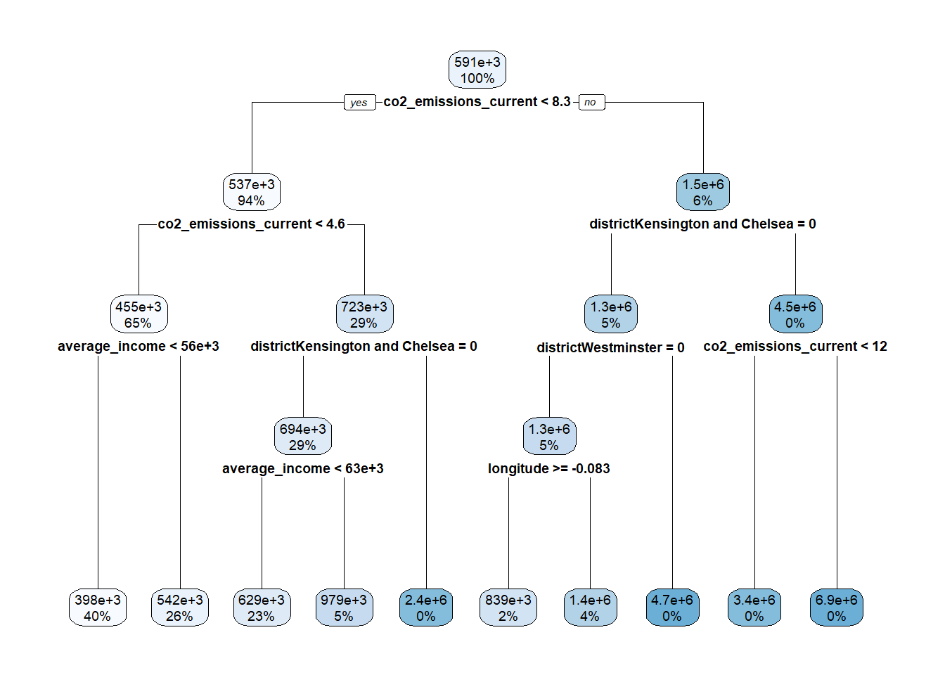
# predict testing values and RMSE
predictions_tree <- predict(base_tree,test_data)

tree_results<-data.frame(RMSE = RMSE(predictions_tree, test_data$price),
                         Rsquare = R2(predictions_tree, test_data$price))

tree_results
## RMSE Rsquare
## 1 379837.7 0.5079072After creating the base tree model, I now proceed to tune the complexity parameter (cp) for the optimal tree model.
Optimal tree (tuning cp) Model
# Plot model metric vs different values of cp (complexity parameter)

#we can display the performance of the tree algorithm as a function of cp
print(base_tree)
## CART
##
## 10498 samples
## 16 predictor
##
## No pre-processing
## Resampling: Cross-Validated (10 fold)
## Summary of sample sizes: 9448, 9448, 9448, 9448, 9448, 9449, ...
## Resampling results across tuning parameters:
##
## cp RMSE Rsquared MAE
## 0.01116344 366490.8 0.4796808 208373.3
## 0.01224143 371350.6 0.4656442 211301.9
## 0.01468396 375630.6 0.4548960 214464.4
## 0.02024850 380978.2 0.4382873 219304.4
## 0.02755995 397833.2 0.3959637 223756.8
## 0.05429934 423868.5 0.3124573 237451.1
## 0.05492236 423868.5 0.3124573 237451.1
## 0.05880129 435576.4 0.2741611 244427.3
## 0.09698212 449051.9 0.2311628 247508.2
## 0.18303499 484315.6 0.1534483 263984.6
##
## RMSE was used to select the optimal model using the smallest value.
## The final value used for the model was cp = 0.01116344.#or plot the results
plot(base_tree)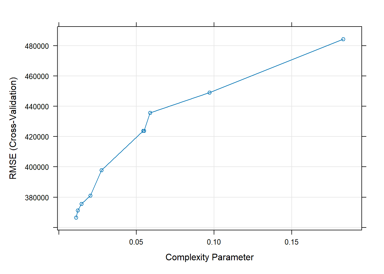
modelLookup("rpart")## model parameter label forReg forClass probModel
## 1 rpart cp Complexity Parameter TRUE TRUE TRUE# Let's set reasonable values for 'cp'
trctrl <- trainControl(method = "cv",
number = 10,
verboseIter = FALSE)
#I choose cp values that seems to result in low error based on plot above
Grid <- expand.grid(cp = seq(0.0000, 0.0030,0.0001))
model2_dtree <- train(price ~ distance_to_station + water_company + property_type + whether_old_or_new + freehold_or_leasehold + latitude + longitude + num_tube_lines + num_rail_lines + num_light_rail_lines + average_income + co2_emissions_current + number_habitable_rooms + district + windows_energy_eff + tenure,
data = train_data,
method = "rpart",
trControl = trctrl,
tuneGrid = Grid)
# Print the search results of 'train' function
plot(model2_dtree) 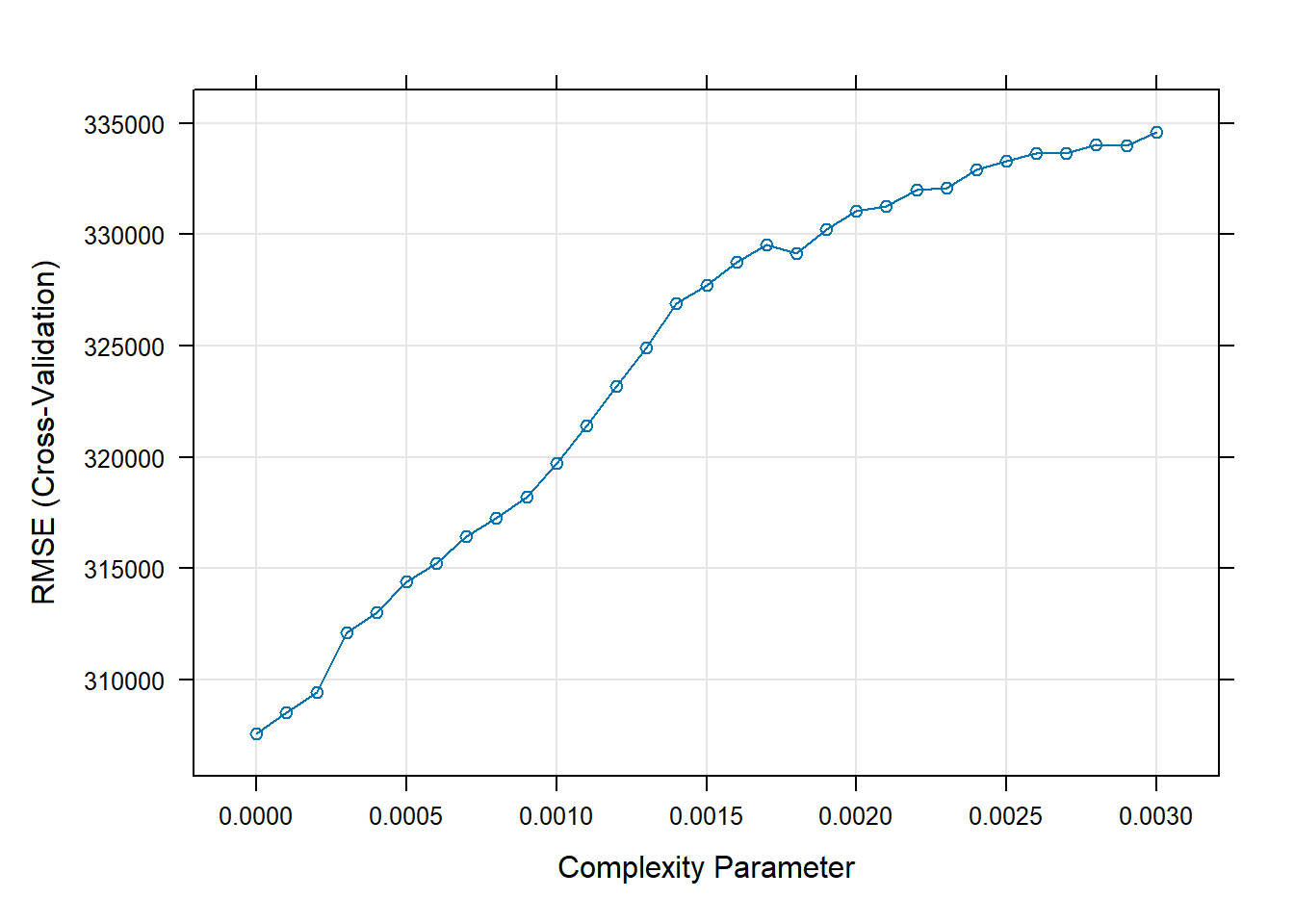
print(model2_dtree)## CART
##
## 10498 samples
## 16 predictor
##
## No pre-processing
## Resampling: Cross-Validated (10 fold)
## Summary of sample sizes: 9448, 9449, 9449, 9448, 9448, 9448, ...
## Resampling results across tuning parameters:
##
## cp RMSE Rsquared MAE
## 0.0000 307548.9 0.6408855 150371.2
## 0.0001 308514.8 0.6371332 151879.7
## 0.0002 309429.1 0.6341573 153901.8
## 0.0003 312095.5 0.6270211 157525.8
## 0.0004 313008.6 0.6244152 159837.1
## 0.0005 314398.8 0.6205542 161915.1
## 0.0006 315230.5 0.6181538 163268.8
## 0.0007 316422.0 0.6148232 164816.9
## 0.0008 317273.6 0.6117584 166017.6
## 0.0009 318190.1 0.6086848 167093.2
## 0.0010 319731.5 0.6049587 168314.9
## 0.0011 321404.8 0.5999050 169414.0
## 0.0012 323202.0 0.5947601 170596.8
## 0.0013 324924.2 0.5906996 171907.4
## 0.0014 326893.6 0.5852883 173780.7
## 0.0015 327713.5 0.5837272 174338.6
## 0.0016 328754.9 0.5809238 175229.9
## 0.0017 329544.1 0.5789256 175714.8
## 0.0018 329168.5 0.5802032 175684.7
## 0.0019 330254.6 0.5772979 176632.8
## 0.0020 331060.4 0.5750468 177315.2
## 0.0021 331256.1 0.5745946 177972.9
## 0.0022 332020.7 0.5723940 179229.4
## 0.0023 332106.9 0.5717783 179912.8
## 0.0024 332912.5 0.5695310 181269.5
## 0.0025 333325.0 0.5689018 181826.8
## 0.0026 333649.7 0.5684444 182112.7
## 0.0027 333663.1 0.5683043 182319.5
## 0.0028 334044.4 0.5672909 182871.4
## 0.0029 334012.5 0.5669230 183087.5
## 0.0030 334620.5 0.5655155 183724.5
##
## RMSE was used to select the optimal model using the smallest value.
## The final value used for the model was cp = 0.# Check variable importance
varImp(model2_dtree)$importance %>%
as.data.frame() %>%
rownames_to_column() %>%
arrange(Overall) %>%
mutate(rowname = forcats::fct_inorder(rowname)) %>%
slice_max(Overall, n = 20) %>%
ggplot()+
geom_col(aes(x = rowname, y = Overall)) +
labs(y = "Importance", x = "") +
coord_flip() +
theme_bw()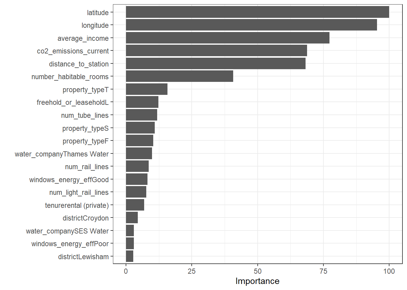
# Calculate testing predictions and RMSE
predictions_dtree_cp <- predict(model2_dtree,test_data)

dtree_cp_results<-data.frame(RMSE = RMSE(predictions_dtree_cp, test_data$price),
                             Rsquare = R2(predictions_dtree_cp, test_data$price))

dtree_cp_results
## RMSE Rsquare
## 1 312083.5 0.6756176KNN Model
set.seed(100)

#knn model
knn <- train(
  price ~ distance_to_station + water_company + property_type + whether_old_or_new + freehold_or_leasehold + latitude + longitude + num_tube_lines + num_rail_lines + num_light_rail_lines + average_income + co2_emissions_current + number_habitable_rooms + district + windows_energy_eff + tenure,
  data = train_data,
  method = "knn",
  trControl = control, #use 10 fold cross validation
  tuneLength = 10, #number of parameter values train function will try
  preProcess = c("center", "scale"))  #center and scale the data in k-nn this is pretty important

knn
## k-Nearest Neighbors ## ## 10498 samples ## 16 predictor ## ## Pre-processing: centered (56), scaled (56) ## Resampling: Cross-Validated (10 fold) ## Summary of sample sizes: 9448, 9448, 9448, 9448, 9448, 9449, ... ## Resampling results across tuning parameters: ## ## k RMSE Rsquared MAE ## 5 315894.0 0.6236477 148163.0 ## 7 310416.8 0.6390899 145849.6 ## 9 311563.5 0.6396419 145441.5 ## 11 307591.6 0.6529652 144650.8 ## 13 309432.2 0.6526569 144845.3 ## 15 312071.5 0.6490910 145393.7 ## 17 312524.9 0.6505576 145515.1 ## 19 314422.8 0.6477354 145870.5 ## 21 315704.8 0.6477728 146372.8 ## 23 316006.0 0.6496556 146983.6 ## ## RMSE was used to select the optimal model using the smallest value. ## The final value used for the model was k = 11.plot(knn) #we can plot the results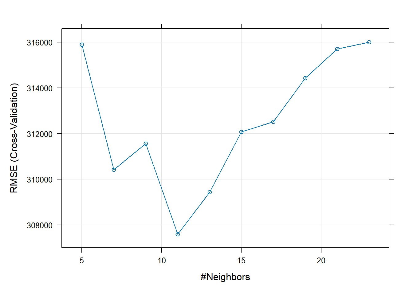
suppressMessages(library(caret))
modelLookup("knn") #It is always a good idea to check the tunable parameters of an algorithm
## model parameter label forReg forClass probModel ## 1 knn k #Neighbors TRUE TRUE TRUE# I will store the values of k I want to experiment with in knnGrid knnGrid <- expand.grid(k= seq(1,100 , by = 5)) # By fixing the see I can re-generate the results when needed set.seed(100) fit_KNN <- train(price ~ distance_to_station + water_company + property_type + whether_old_or_new + freehold_or_leasehold + latitude + longitude + num_tube_lines + num_rail_lines + num_light_rail_lines + average_income + co2_emissions_current + number_habitable_rooms + district + windows_energy_eff + tenure, data=train_data, preProcess = c("center", "scale"), method="knn", trControl=control, tuneGrid = knnGrid) # display results print(fit_KNN)## k-Nearest Neighbors ## ## 10498 samples ## 16 predictor ## ## Pre-processing: centered (56), scaled (56) ## Resampling: Cross-Validated (10 fold) ## Summary of sample sizes: 9448, 9448, 9448, 9448, 9448, 9449, ... ## Resampling results across tuning parameters: ## ## k RMSE Rsquared MAE ## 1 369713.1 0.5111213 174739.0 ## 6 310998.4 0.6354419 146117.4 ## 11 307591.6 0.6529652 144650.8 ## 16 312511.4 0.6492891 145396.6 ## 21 315704.8 0.6477728 146372.8 ## 26 318886.9 0.6450050 147874.5 ## 31 323713.5 0.6383297 149655.0 ## 36 327072.6 0.6355140 151204.2 ## 41 331829.3 0.6280102 152663.7 ## 46 336349.1 0.6209301 154387.1 ## 51 340288.8 0.6135423 156026.0 ## 56 343714.0 0.6080812 157805.0 ## 61 347236.9 0.6019403 159265.6 ## 66 351205.8 0.5936074 161049.6 ## 71 354363.9 0.5874348 162466.3 ## 76 357887.5 0.5791140 164224.0 ## 81 360719.2 0.5726815 165775.2 ## 86 363713.4 0.5653187 167177.0 ## 91 366764.9 0.5576986 168777.4 ## 96 369853.2 0.5482934 170508.8 ## ## RMSE was used to select the optimal model using the smallest value. ## The final value used for the model was k = 11.# plot results plot(fit_KNN)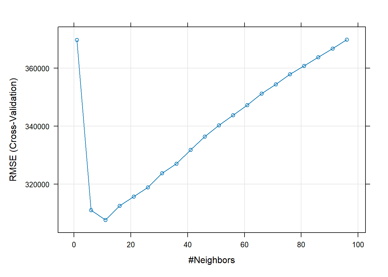
# Try a subsetted grid after seeing the plot
knnGrid_subset <-  expand.grid(k= seq(6,16 , by = 1))

set.seed(100)
model3_knn <- train(price ~ distance_to_station + water_company + property_type + whether_old_or_new + freehold_or_leasehold + latitude + longitude + num_tube_lines + num_rail_lines + num_light_rail_lines + average_income + co2_emissions_current + number_habitable_rooms + district + windows_energy_eff + tenure,
  data = train_data,
                 preProcess = c("center", "scale"),
                 method="knn",
                 trControl=control,
                 tuneGrid = knnGrid_subset)

# display results
print(model3_knn)
## k-Nearest Neighbors ## ## 10498 samples ## 16 predictor ## ## Pre-processing: centered (56), scaled (56) ## Resampling: Cross-Validated (10 fold) ## Summary of sample sizes: 9448, 9448, 9448, 9448, 9448, 9449, ... ## Resampling results across tuning parameters: ## ## k RMSE Rsquared MAE ## 6 310998.4 0.6354419 146117.4 ## 7 310416.8 0.6390899 145849.6 ## 8 311085.3 0.6392452 145341.2 ## 9 311563.5 0.6396419 145441.5 ## 10 309808.8 0.6455951 144917.9 ## 11 307591.6 0.6529652 144650.8 ## 12 308605.8 0.6529274 144658.9 ## 13 309432.2 0.6526569 144845.3 ## 14 310459.4 0.6517043 145007.4 ## 15 312071.5 0.6490910 145393.7 ## 16 312511.4 0.6492891 145396.6 ## ## RMSE was used to select the optimal model using the smallest value. ## The final value used for the model was k = 11.# plot results plot(model3_knn)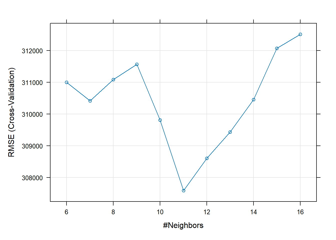
# I can now confirm that k = 11 is the optimal number of nearest neighbours for lowest validation RMSE

# Calculate testing Wpredictions and RMSE
predictions_knn <- predict(model3_knn,test_data)

knn_results<-data.frame(RMSE = RMSE(predictions_knn, test_data$price),
                        Rsquare = R2(predictions_knn, test_data$price))

knn_results
## RMSE Rsquare ## 1 301321.8 0.7124816# # we can check variable importance as well # varImp(model3_knn)$importance %>% # as.data.frame() %>% # rownames_to_column() %>% # arrange(Overall) %>% # mutate(rowname = forcats::fct_inorder(rowname)) %>% # slice_max(Overall, n = 20) %>% # ggplot()+ # geom_col(aes(x = rowname, y = Overall)) + # labs(y = "Importance", x = "") + # coord_flip() + # theme_bw()
LASSO Model
lambda_seq <- seq(0, 0.01, length = 1000)

# lasso regression using k-fold cross validation to select the best lambda
set.seed(100)
model4_lasso <- train(
  price ~ distance_to_station + water_company + property_type + whether_old_or_new + freehold_or_leasehold + latitude + longitude + num_tube_lines + num_rail_lines + num_light_rail_lines + average_income + co2_emissions_current + number_habitable_rooms + district + windows_energy_eff + tenure,
 data = train_data,
 method = "glmnet",
  preProc = c("center", "scale"), #This option standardizes the data before running the LASSO regression
  trControl = control,
  tuneGrid = expand.grid(alpha = 1, lambda = lambda_seq) #alpha=1 specifies to run a LASSO regression.
  )

# Model coefficients
coef(model4_lasso$finalModel, model4_lasso$bestTune$lambda)
## 57 x 1 sparse Matrix of class "dgCMatrix"
## s1
## (Intercept) 590665.5545
## distance_to_station -7006.3762
## water_companyEssex & Suffolk Water 6803.4291
## water_companyLeep Utilities 1438.0513
## water_companySES Water 10733.2424
## water_companyThames Water 66135.2629
## property_typeF -26343.0009
## property_typeS -32910.2356
## property_typeT -12449.9434
## whether_old_or_newY 2721.9160
## freehold_or_leaseholdL -7212.7867
## latitude 46366.4352
## longitude 69895.3177
## num_tube_lines 24758.4806
## num_rail_lines 3908.1141
## num_light_rail_lines 6528.5283
## average_income 81838.0807
## co2_emissions_current 152784.5516
## number_habitable_rooms 146150.5907
## districtBarnet 24680.7975
## districtBexley -33607.5527
## districtBrent 37613.4590
## districtBromley -15257.2095
## districtCamden 60130.4021
## districtCity of London 7287.6606
## districtCroydon 1498.2958
## districtEaling 32176.5392
## districtEnfield -16343.6808
## districtGreenwich -6821.0388
## districtHackney 33271.9579
## districtHammersmith and Fulham 64695.8700
## districtHaringey 12334.6025
## districtHarrow 17203.4029
## districtHavering -26284.2000
## districtHillingdon 37092.1067
## districtHounslow 33908.3054
## districtIslington 42804.4271
## districtKensington and Chelsea 172611.8586
## districtKingston upon Thames 27253.4696
## districtLambeth 30489.4024
## districtLewisham 2548.2648
## districtMerton 24168.7224
## districtNewham -10625.8914
## districtRedbridge -26836.8387
## districtRichmond upon Thames 48202.6116
## districtSouthwark 36068.7228
## districtSutton 21833.7986
## districtTower Hamlets 16476.0776
## districtWaltham Forest -6830.0347
## districtWandsworth 44139.3235
## districtWestminster 109037.6933
## windows_energy_effGood 25490.1624
## windows_energy_effPoor 14700.3830
## windows_energy_effVery Good -944.8076
## windows_energy_effVery Poor -2795.6608
## tenurerental (private) -8799.7168
## tenurerental (social) -1684.6359# Best lambda
model4_lasso$bestTune$lambda## [1] 0.01# Count of how many coefficients are greater than zero and how many are equal to zero
sum(coef(model4_lasso$finalModel, model4_lasso$bestTune$lambda)!=0)## [1] 57sum(coef(model4_lasso$finalModel, model4_lasso$bestTune$lambda)==0)## [1] 0# Make predictions
predictions_lasso <- predict(model4_lasso, test_data)
# Model prediction performance
lasso_results <- data.frame(RMSE = RMSE(predictions_lasso, test_data$price),
Rsquare = R2(predictions_lasso, test_data$price))
lasso_results## RMSE Rsquare
## 1 333198.1 0.6187213# we can check variable importance as well
varImp(model4_lasso)$importance %>%
as.data.frame() %>%
rownames_to_column() %>%
arrange(Overall) %>%
mutate(rowname = forcats::fct_inorder(rowname)) %>%
slice_max(Overall, n = 20) %>%
ggplot()+
geom_col(aes(x = rowname, y = Overall)) +
labs(y = "Importance", x = "") +
coord_flip() +
theme_bw()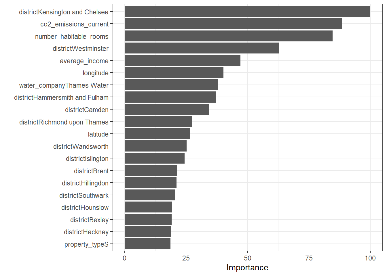
Random Forest Model
# The following function gives the list of tunable parameters
modelLookup("ranger")
## model parameter label forReg forClass probModel
## 1 ranger mtry #Randomly Selected Predictors TRUE TRUE TRUE
## 2 ranger splitrule Splitting Rule TRUE TRUE TRUE
## 3 ranger min.node.size Minimal Node Size TRUE TRUE TRUE# Define the tuning grid: tuneGrid
# Let's do a search on 'mtry'; number of variables to use in each split
gridRF <- data.frame(
.mtry = c(2:7),
.splitrule = "variance",
.min.node.size = 5
)
set.seed(100)
# Fit random forest: model= ranger using caret library anf train function
model5_rf <- train(
price ~ distance_to_station + water_company + property_type + whether_old_or_new + freehold_or_leasehold + latitude + longitude + num_tube_lines + num_rail_lines + num_light_rail_lines + average_income + co2_emissions_current + number_habitable_rooms + district + windows_energy_eff + tenure,
data = train_data,
method = "ranger",
trControl = control,
tuneGrid = gridRF,
importance = 'permutation'
#This is the method used to determine variable importance.
#Permutation=leave one variable out and fit the model again
)
# Print model to console
varImp(model5_rf)## ranger variable importance
##
## only 20 most important variables shown (out of 56)
##
## Overall
## number_habitable_rooms 100.000
## co2_emissions_current 91.490
## districtKensington and Chelsea 68.088
## freehold_or_leaseholdL 61.976
## num_tube_lines 58.375
## longitude 56.511
## property_typeF 54.151
## latitude 49.263
## average_income 42.183
## districtWestminster 29.314
## water_companyThames Water 23.958
## num_rail_lines 14.581
## property_typeT 12.603
## distance_to_station 11.791
## property_typeS 5.899
## num_light_rail_lines 5.488
## districtHammersmith and Fulham 4.497
## districtCamden 3.839
## districtWandsworth 3.414
## water_companyEssex & Suffolk Water 2.804plot(varImp(model5_rf))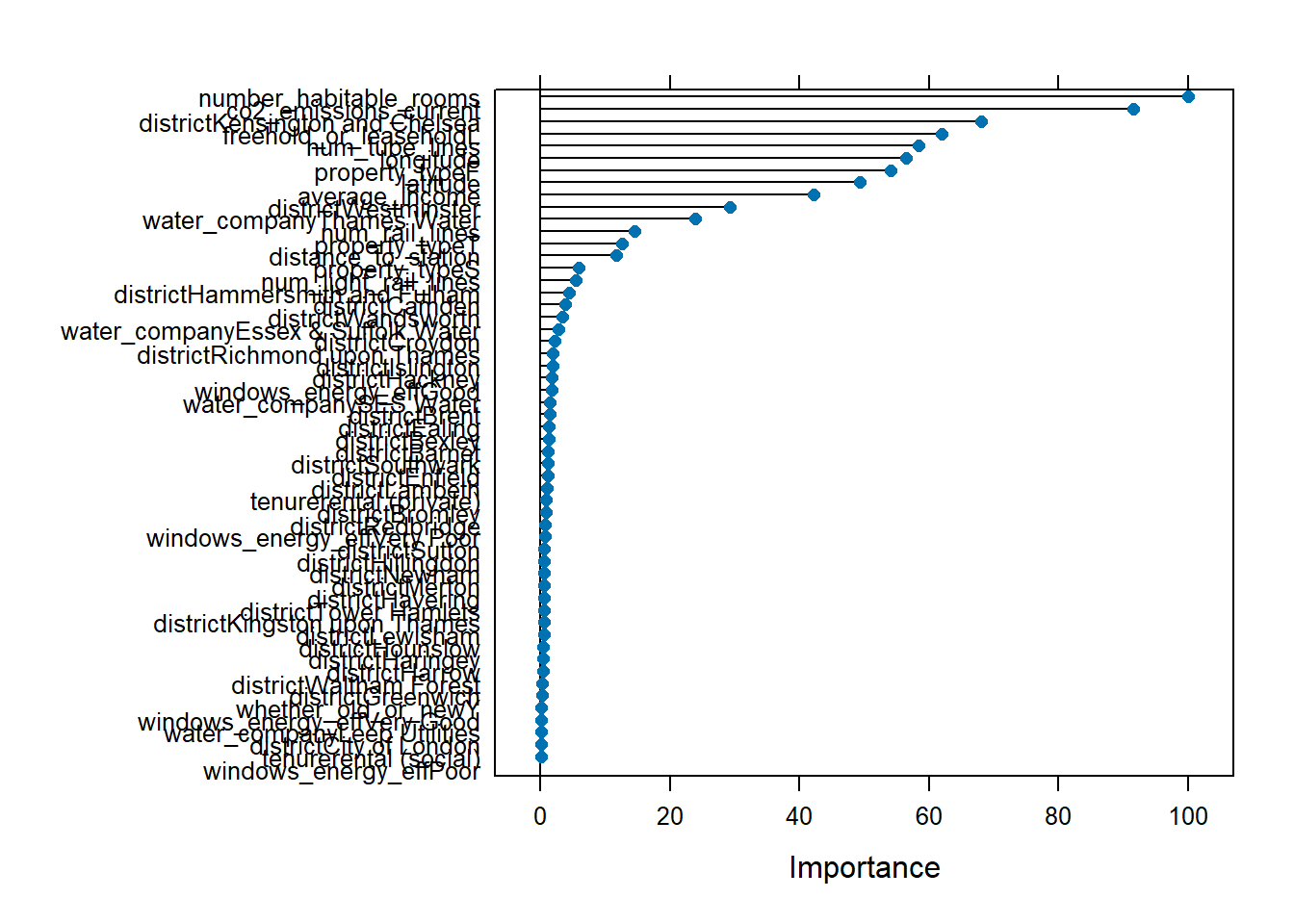
summary(model5_rf)## Length Class Mode
## predictions 10498 -none- numeric
## num.trees 1 -none- numeric
## num.independent.variables 1 -none- numeric
## mtry 1 -none- numeric
## min.node.size 1 -none- numeric
## variable.importance 56 -none- numeric
## prediction.error 1 -none- numeric
## forest 7 ranger.forest list
## splitrule 1 -none- character
## treetype 1 -none- character
## r.squared 1 -none- numeric
## call 9 -none- call
## importance.mode 1 -none- character
## num.samples 1 -none- numeric
## replace 1 -none- logical
## dependent.variable.name 1 -none- character
## xNames 56 -none- character
## problemType 1 -none- character
## tuneValue 3 data.frame list
## obsLevels 1 -none- logical
## param 1 -none- listprint(model5_rf)## Random Forest
##
## 10498 samples
## 16 predictor
##
## No pre-processing
## Resampling: Cross-Validated (10 fold)
## Summary of sample sizes: 9448, 9448, 9448, 9448, 9448, 9449, ...
## Resampling results across tuning parameters:
##
## mtry RMSE Rsquared MAE
## 2 362571.2 0.6634160 174943.4
## 3 318412.4 0.7010216 148733.2
## 4 294524.1 0.7235003 135752.5
## 5 278985.8 0.7400105 128384.7
## 6 271544.0 0.7470752 124415.4
## 7 266468.8 0.7506937 122089.8
##
## Tuning parameter 'splitrule' was held constant at a value of variance
##
## Tuning parameter 'min.node.size' was held constant at a value of 5
## RMSE was used to select the optimal model using the smallest value.
## The final values used for the model were mtry = 7, splitrule = variance
## and min.node.size = 5.# Calculate testing predictions and RMSE
predictions_rf <- predict(model5_rf, test_data)
rf_results<-data.frame(RMSE = RMSE(predictions_rf, test_data$price),
Rsquare = R2(predictions_rf, test_data$price))
rf_results## RMSE Rsquare
## 1 255588 0.7903486# check variable importance
varImp(model5_rf)$importance %>%
as.data.frame() %>%
rownames_to_column() %>%
arrange(Overall) %>%
mutate(rowname = forcats::fct_inorder(rowname)) %>%
slice_max(Overall, n = 20) %>%
ggplot()+
geom_col(aes(x = rowname, y = Overall)) +
labs(y = "Importance", x = "") +
coord_flip() +
theme_bw()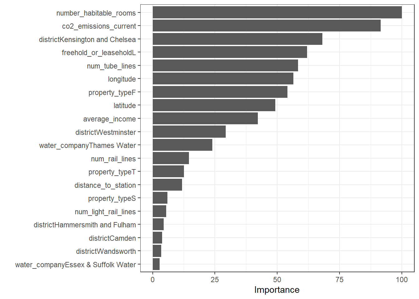
Gradient Boosting Model
modelLookup("gbm")## model parameter label forReg forClass probModel
## 1 gbm n.trees # Boosting Iterations TRUE TRUE TRUE
## 2 gbm interaction.depth Max Tree Depth TRUE TRUE TRUE
## 3 gbm shrinkage Shrinkage TRUE TRUE TRUE
## 4 gbm n.minobsinnode Min. Terminal Node Size TRUE TRUE TRUE#Expand the search grid (see above for definitions)
grid<-expand.grid(interaction.depth = c(3:7), n.trees = seq(150,250,10), shrinkage = 0.075, n.minobsinnode = 10)
set.seed(100)
#Train for gbm
model6_gbm <- train(price ~ distance_to_station + water_company + property_type + whether_old_or_new + freehold_or_leasehold + latitude + longitude + num_tube_lines + num_rail_lines + num_light_rail_lines + average_income + co2_emissions_current + number_habitable_rooms + district + windows_energy_eff + tenure,
data = train_data,
method = "gbm",
trControl = control,
tuneGrid = grid,
verbose = FALSE
)
print(model6_gbm)## Stochastic Gradient Boosting
##
## 10498 samples
## 16 predictor
##
## No pre-processing
## Resampling: Cross-Validated (10 fold)
## Summary of sample sizes: 9448, 9448, 9448, 9448, 9448, 9449, ...
## Resampling results across tuning parameters:
##
## interaction.depth n.trees RMSE Rsquared MAE
## 3 150 279189.4 0.7020344 138286.1
## 3 160 278689.9 0.7033182 137640.3
## 3 170 278264.5 0.7043799 137297.3
## 3 180 277337.5 0.7062178 136449.1
## 3 190 276614.6 0.7080378 135878.5
## 3 200 275538.2 0.7103785 135363.8
## 3 210 274479.9 0.7121032 134831.6
## 3 220 273691.7 0.7137876 134472.6
## 3 230 273181.8 0.7143834 134248.2
## 3 240 272363.2 0.7159365 134005.8
## 3 250 272183.5 0.7163864 133779.9
## 4 150 274009.4 0.7126546 133691.7
## 4 160 273779.5 0.7140519 133124.8
## 4 170 273255.3 0.7150010 132738.2
## 4 180 272225.6 0.7167975 132245.1
## 4 190 270593.0 0.7191123 131719.6
## 4 200 269835.2 0.7210569 131528.1
## 4 210 268755.7 0.7228706 131028.7
## 4 220 267823.2 0.7246752 130702.1
## 4 230 267214.2 0.7258803 130422.2
## 4 240 266805.6 0.7264685 130266.3
## 4 250 266991.8 0.7261998 130210.8
## 5 150 265664.7 0.7295790 130310.9
## 5 160 265120.2 0.7309764 129907.6
## 5 170 264623.4 0.7319259 129524.0
## 5 180 264175.1 0.7328710 129337.2
## 5 190 263279.0 0.7344643 128880.3
## 5 200 262897.9 0.7352268 128592.2
## 5 210 262229.6 0.7361963 128367.9
## 5 220 261623.8 0.7373652 127981.8
## 5 230 261233.2 0.7381577 127750.0
## 5 240 260855.6 0.7391343 127638.7
## 5 250 260676.0 0.7397150 127463.7
## 6 150 265198.8 0.7331515 128635.8
## 6 160 264366.6 0.7353427 128141.5
## 6 170 263016.8 0.7375622 127623.4
## 6 180 260952.3 0.7409010 127084.6
## 6 190 260592.4 0.7418974 126973.8
## 6 200 260429.1 0.7423683 126823.4
## 6 210 259857.8 0.7434063 126674.2
## 6 220 259518.5 0.7443708 126412.5
## 6 230 258172.2 0.7462838 126092.5
## 6 240 257689.0 0.7465244 125883.9
## 6 250 257583.2 0.7467868 125903.9
## 7 150 262130.4 0.7379771 127415.5
## 7 160 260950.2 0.7400268 126957.3
## 7 170 261098.8 0.7397685 126748.3
## 7 180 260415.0 0.7410419 126440.8
## 7 190 259872.7 0.7418367 126061.9
## 7 200 259384.8 0.7427716 125756.4
## 7 210 259637.4 0.7424211 125673.0
## 7 220 257950.6 0.7455616 125192.2
## 7 230 256651.5 0.7477667 124863.0
## 7 240 256517.7 0.7482415 124790.1
## 7 250 256163.3 0.7491068 124557.9
##
## Tuning parameter 'shrinkage' was held constant at a value of 0.075
##
## Tuning parameter 'n.minobsinnode' was held constant at a value of 10
## RMSE was used to select the optimal model using the smallest value.
## The final values used for the model were n.trees = 250, interaction.depth =
## 7, shrinkage = 0.075 and n.minobsinnode = 10.# Calculate testing predictions and RMSE
predictions_boost = predict(model6_gbm, test_data)
boost_results<-data.frame(RMSE = RMSE(predictions_boost, test_data$price),
Rsquare = R2(predictions_boost, test_data$price))
boost_results ## RMSE Rsquare
## 1 253037 0.7798198# # check variable importance
# varImp(model6_gbm, numTrees = 250)$importance %>%
# as.data.frame() %>%
# rownames_to_column() %>%
# arrange(Overall) %>%
# mutate(rowname = forcats::fct_inorder(rowname)) %>%
# slice_max(Overall, n = 20) %>%
# ggplot()+
# geom_col(aes(x = rowname, y = Overall)) +
# labs(y = "Importance", x = "") +
# coord_flip() +
# theme_bw()
# set.seed(100)
# boost.fit <- gbm(price ~ distance_to_station + water_company + property_type + whether_old_or_new + freehold_or_leasehold + latitude + longitude + num_tube_lines + num_rail_lines + num_light_rail_lines + average_income + co2_emissions_current + number_habitable_rooms + district + windows_energy_eff + tenure,
# data = train_data,
# distribution = "gaussian",
# interaction.depth = 6,n.trees = 10000,shrinkage = 0.075, n.minobsinnode = 10, cv.folds = 10
# )
#
# print(boost.fit)
#
# bestoob = gbm.perf(boost.fit, method = "OOB")
# bestoob
#
#
# boostoob.pred = predict(boost.fit, newdata = test_data, n.trees = bestoob, type = "response")
#
# oobboost_results<-data.frame(RMSE = RMSE(boostoob.pred, test_data$price),
# Rsquare = R2(boostoob.pred, test_data$price))
#
# oobboost_results xgBoost Model
Here, I try an xgboost model to compare how another version of gradient boosting measures up against its counterpart.
library(xgboost)##
## Attaching package: 'xgboost'## The following object is masked from 'package:dplyr':
##
## slicetrainlabels = train_data$price
testlabels = test_data$price
train_matrix <- train_data %>%
select(c(distance_to_station, water_company, property_type, whether_old_or_new, freehold_or_leasehold, latitude, longitude, num_tube_lines, num_rail_lines, num_light_rail_lines, average_income, co2_emissions_current, number_habitable_rooms, district, windows_energy_eff, tenure
)) %>%
data.matrix(.)
dtrain = xgb.DMatrix(data = train_matrix, label = trainlabels)
test_matrix <- test_data %>%
select(c(distance_to_station, water_company, property_type, whether_old_or_new, freehold_or_leasehold, latitude, longitude, num_tube_lines, num_rail_lines, num_light_rail_lines, average_income, co2_emissions_current, number_habitable_rooms, district, windows_energy_eff, tenure
)) %>%
data.matrix(.)
dtest = xgb.DMatrix(data = test_matrix, label = testlabels)
model7_xgboost = xgboost(data = dtrain, max.depth = 3, nrounds = 99, objective = "reg:squarederror", eval_metric = "rmse")## [1] train-rmse:614713.026168
## [2] train-rmse:509919.453240
## [3] train-rmse:439187.235794
## [4] train-rmse:394540.013681
## [5] train-rmse:365852.911401
## [6] train-rmse:344637.202589
## [7] train-rmse:330487.727236
## [8] train-rmse:319417.618464
## [9] train-rmse:311482.183758
## [10] train-rmse:302204.184423
## [11] train-rmse:297626.216966
## [12] train-rmse:292333.761183
## [13] train-rmse:288436.744246
## [14] train-rmse:284755.683924
## [15] train-rmse:281328.064582
## [16] train-rmse:276019.610225
## [17] train-rmse:274000.468189
## [18] train-rmse:271926.277255
## [19] train-rmse:270015.801869
## [20] train-rmse:268642.509132
## [21] train-rmse:265356.799457
## [22] train-rmse:260841.795488
## [23] train-rmse:259110.613893
## [24] train-rmse:258072.683474
## [25] train-rmse:256875.584297
## [26] train-rmse:255507.410083
## [27] train-rmse:254439.164547
## [28] train-rmse:253886.002887
## [29] train-rmse:252848.151811
## [30] train-rmse:251838.695776
## [31] train-rmse:250250.988417
## [32] train-rmse:249291.988908
## [33] train-rmse:248596.802268
## [34] train-rmse:247907.248348
## [35] train-rmse:246655.948310
## [36] train-rmse:242211.467281
## [37] train-rmse:241304.007182
## [38] train-rmse:240675.263223
## [39] train-rmse:240163.440829
## [40] train-rmse:239629.798766
## [41] train-rmse:238806.591963
## [42] train-rmse:238081.691798
## [43] train-rmse:237595.237673
## [44] train-rmse:234766.118942
## [45] train-rmse:233930.059440
## [46] train-rmse:233592.848436
## [47] train-rmse:233181.298273
## [48] train-rmse:232446.392453
## [49] train-rmse:231358.156523
## [50] train-rmse:230028.367758
## [51] train-rmse:229703.268396
## [52] train-rmse:229188.047290
## [53] train-rmse:228763.479352
## [54] train-rmse:227249.340861
## [55] train-rmse:226518.835159
## [56] train-rmse:225434.445224
## [57] train-rmse:225122.243699
## [58] train-rmse:224843.210769
## [59] train-rmse:224437.337225
## [60] train-rmse:223761.831479
## [61] train-rmse:222755.584441
## [62] train-rmse:222383.098686
## [63] train-rmse:221905.149295
## [64] train-rmse:220837.291253
## [65] train-rmse:220626.660436
## [66] train-rmse:220160.911458
## [67] train-rmse:219956.779844
## [68] train-rmse:218637.431014
## [69] train-rmse:218395.678318
## [70] train-rmse:217823.866238
## [71] train-rmse:217550.446629
## [72] train-rmse:216799.725243
## [73] train-rmse:216030.866504
## [74] train-rmse:215442.727521
## [75] train-rmse:215166.112867
## [76] train-rmse:214420.476695
## [77] train-rmse:214031.066258
## [78] train-rmse:213825.724573
## [79] train-rmse:213680.210307
## [80] train-rmse:213444.210751
## [81] train-rmse:212971.150301
## [82] train-rmse:212630.019966
## [83] train-rmse:211257.871233
## [84] train-rmse:210679.848674
## [85] train-rmse:209993.731404
## [86] train-rmse:209569.892306
## [87] train-rmse:208687.440291
## [88] train-rmse:208500.669360
## [89] train-rmse:208004.340970
## [90] train-rmse:207759.765176
## [91] train-rmse:207442.881863
## [92] train-rmse:206726.332154
## [93] train-rmse:206379.183391
## [94] train-rmse:206112.351556
## [95] train-rmse:205860.497299
## [96] train-rmse:205692.320125
## [97] train-rmse:204960.210297
## [98] train-rmse:204672.637569
## [99] train-rmse:204441.623549predictions_xgboost = predict(model7_xgboost, dtest)
xgboost_results<-data.frame(RMSE = RMSE(predictions_xgboost, test_data$price),
Rsquare = R2(predictions_xgboost, test_data$price))
xgboost_results## RMSE Rsquare
## 1 288282.4 0.728393RMSE result tabulation
overall_results <- rbind(lr_results, dtree_cp_results, knn_results, lasso_results, rf_results, boost_results, xgboost_results)
rownames(overall_results) = c("linear", "cp tree", "knn", "lasso", "rf", "gbm", "xgboost")

overall_results
## RMSE Rsquare
## linear 333122.5 0.6187907
## cp tree 312083.5 0.6756176
## knn 301321.8 0.7124816
## lasso 333198.1 0.6187213
## rf 255588.0 0.7903486
## gbm 253037.0 0.7798198
## xgboost 288282.4 0.7283930Gradient boosting model is the clear winner here.
Stacking
Use stacking to ensemble your algorithms.
library("caretEnsemble")
my_control <- trainControl(
    method = "cv",
    number = 10,
    savePredictions="final",
    verboseIter = FALSE
  )

#To implement stacking first train all the models you will use
set.seed(100)
model_list <- caretList(
  price ~ distance_to_station + water_company + property_type + whether_old_or_new + freehold_or_leasehold + latitude + longitude + num_tube_lines + num_rail_lines + num_light_rail_lines + average_income + co2_emissions_current + number_habitable_rooms + district + windows_energy_eff + tenure,
  data = train_data,
  trControl = my_control, #Control options
  methodList = c("glm"), # Models in stacking: glm=logistic regression
  tuneList = list(
    knn = caretModelSpec(method = "knn", tuneGrid = data.frame(k = 11), verbose = FALSE), #knn with tuned parameters
    gbm = caretModelSpec(method = "gbm", tuneGrid = data.frame(interaction.depth = 7, n.trees = 250,shrinkage = 0.075, n.minobsinnode = 10), verbose = FALSE), #gbm with tuned parameters
    ranger = caretModelSpec(method="ranger", tuneGrid = data.frame(mtry = 7, splitrule = "variance", min.node.size = 5)), #Random forest with tuned parameters
    rpart = caretModelSpec(method = "rpart", tuneGrid = data.frame(cp = 0))) #Tree with tuned parameters
  )


#Let's look at what information is kept in model_list
  typeof(model_list)
## [1] "list" summary(model_list)## Length Class Mode
## knn 25 train list
## gbm 25 train list
## ranger 25 train list
## rpart 25 train list
## glm 25 train list#Check ranger model for example
summary(model_list$ranger)## Length Class Mode
## predictions 10498 -none- numeric
## num.trees 1 -none- numeric
## num.independent.variables 1 -none- numeric
## mtry 1 -none- numeric
## min.node.size 1 -none- numeric
## prediction.error 1 -none- numeric
## forest 7 ranger.forest list
## splitrule 1 -none- character
## treetype 1 -none- character
## r.squared 1 -none- numeric
## call 9 -none- call
## importance.mode 1 -none- character
## num.samples 1 -none- numeric
## replace 1 -none- logical
## dependent.variable.name 1 -none- character
## xNames 56 -none- character
## problemType 1 -none- character
## tuneValue 3 data.frame list
## obsLevels 1 -none- logical
## param 0 -none- list typeof(model_list$ranger)## [1] "list" print(model_list$ranger$bestTune)## mtry splitrule min.node.size
## 1 7 variance 5# Fortunately caret package has various functions to display relative performance of multiple methods
# To use them we need to put all results together in a list first
resamples <- resamples(model_list)
typeof(resamples)## [1] "list" summary(resamples)##
## Call:
## summary.resamples(object = resamples)
##
## Models: knn, gbm, ranger, rpart, glm
## Number of resamples: 10
##
## MAE
## Min. 1st Qu. Median Mean 3rd Qu. Max. NA's
## knn 156476.8 161442.5 170787.7 170480.5 177349.0 185086.2 0
## gbm 114033.2 122762.7 124080.9 124425.9 127883.5 133007.8 0
## ranger 113473.1 116895.9 120561.7 121618.9 128096.1 130195.2 0
## rpart 139338.4 144601.3 150896.8 150201.7 155431.2 159870.7 0
## glm 160947.8 170370.3 174609.2 174917.0 182240.2 188417.7 0
##
## RMSE
## Min. 1st Qu. Median Mean 3rd Qu. Max. NA's
## knn 302481.8 311500.3 348834.0 373068.0 438746.1 468965.1 0
## gbm 204552.2 223257.4 242791.2 255323.4 295644.7 308454.1 0
## ranger 213557.2 219725.0 239602.0 263705.8 313331.9 342202.9 0
## rpart 249969.6 276620.2 315416.6 307745.4 336227.7 371476.5 0
## glm 275900.2 282498.8 304128.5 334697.5 398437.4 418989.8 0
##
## Rsquared
## Min. 1st Qu. Median Mean 3rd Qu. Max. NA's
## knn 0.4435085 0.4554301 0.4859643 0.5018228 0.5122828 0.6547823 0
## gbm 0.7061618 0.7313497 0.7683644 0.7568211 0.7854610 0.7987169 0
## ranger 0.7092349 0.7353117 0.7610436 0.7592368 0.7891896 0.8027879 0
## rpart 0.5533958 0.6119607 0.6607147 0.6506768 0.6905950 0.7319945 0
## glm 0.5034816 0.5299434 0.5933514 0.5763016 0.6094681 0.6336588 0# We can use dotplots
dotplot(resamples)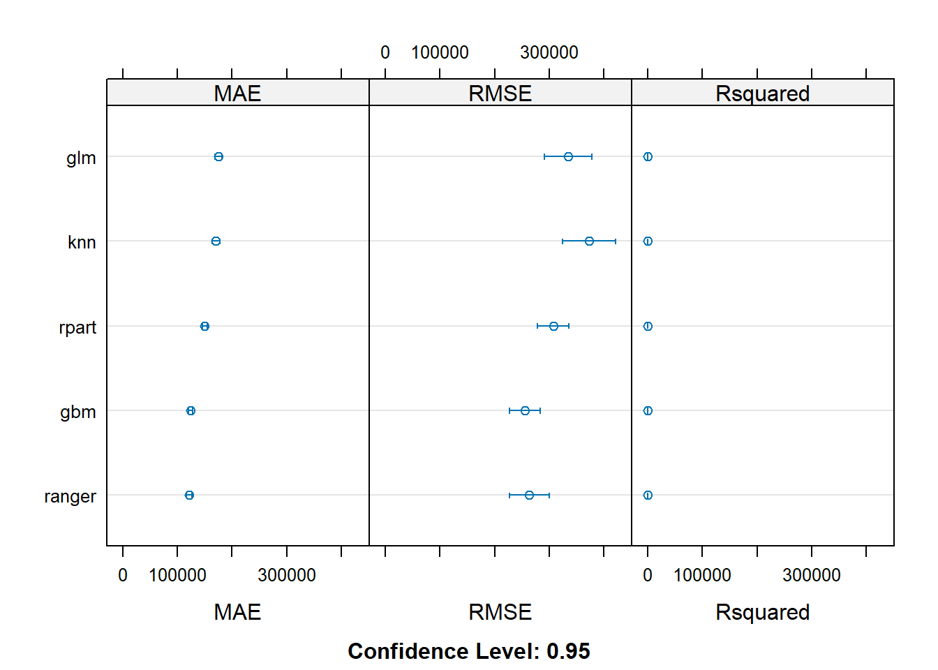
# We can use box plots
bwplot(resamples) 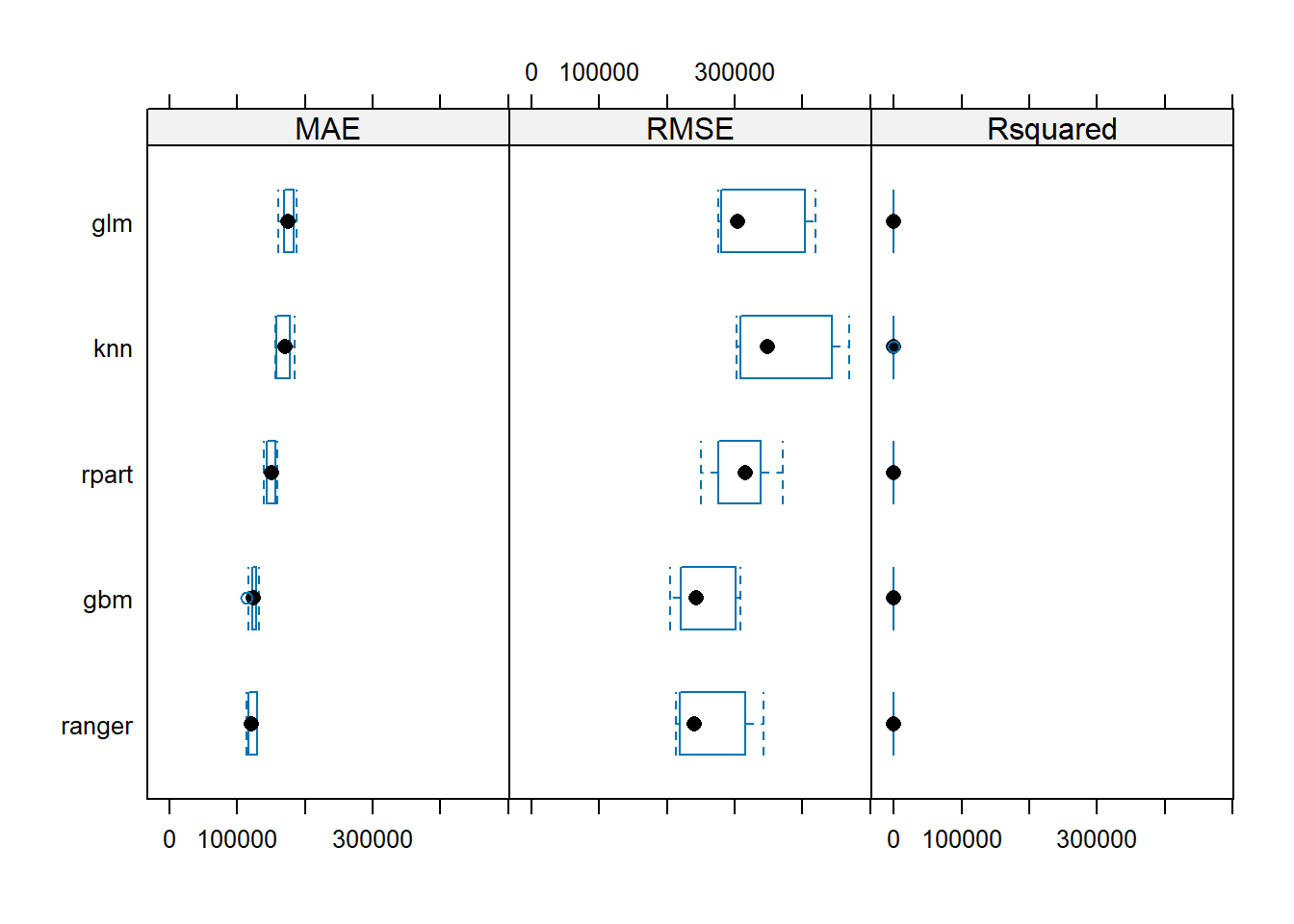
#or correlations
  modelCor(resamples)
## knn gbm ranger rpart glm
## knn 1.0000000 0.8145980 0.9042818 0.6791909 0.8822695
## gbm 0.8145980 1.0000000 0.8880856 0.8359400 0.9146193
## ranger 0.9042818 0.8880856 1.0000000 0.7729849 0.9648449
## rpart 0.6791909 0.8359400 0.7729849 1.0000000 0.7313484
## glm 0.8822695 0.9146193 0.9648449 0.7313484 1.0000000#We can visualize results in scatter plots as well
splom(resamples)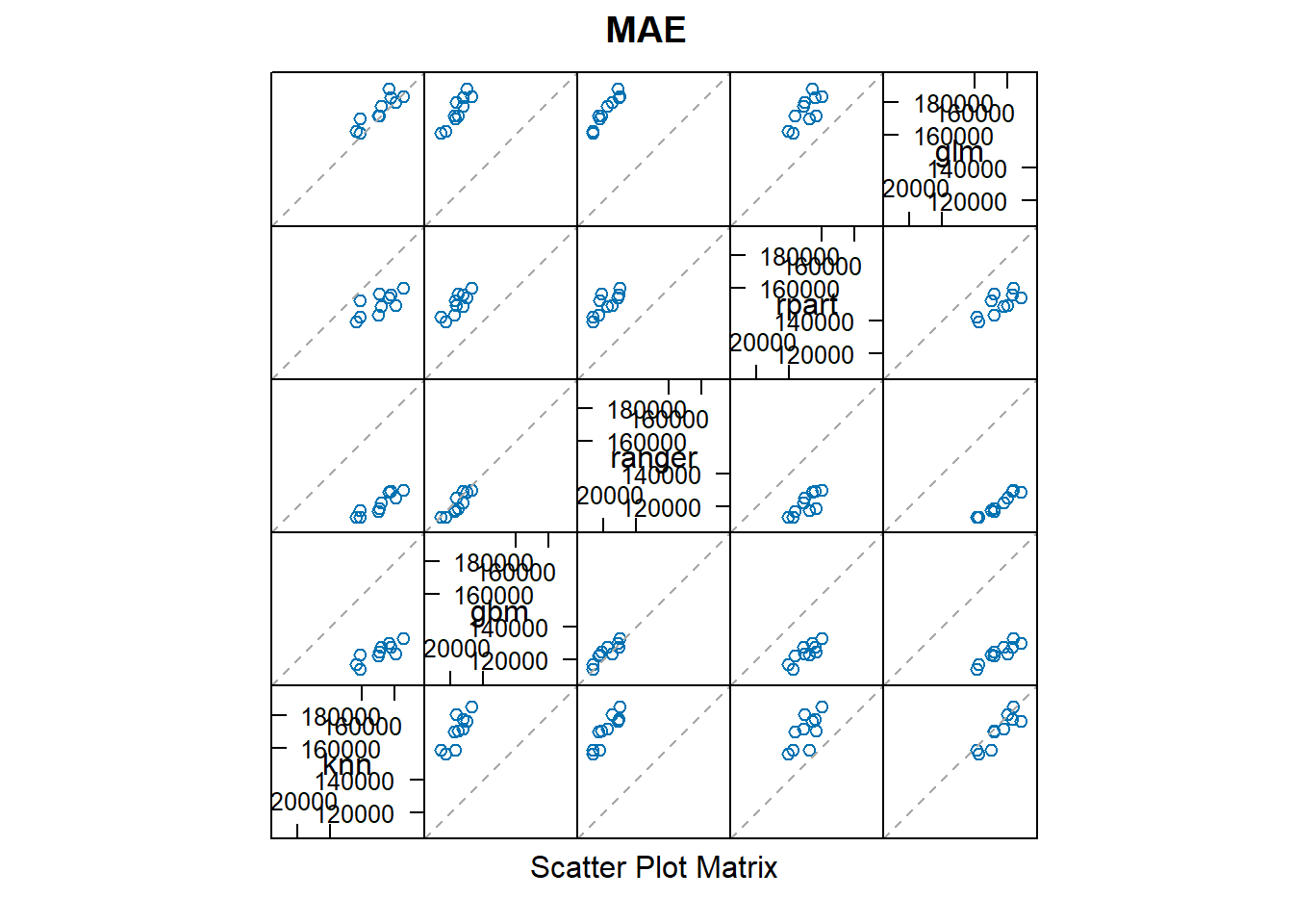
#Now we can put all the results together and stack them
glm_ensemble <- caretStack(
    model_list, #Models we trained above in caretList
    method = "glm", #Use logistic regression to combine
    trControl = my_control
  )

  summary(glm_ensemble)
##
## Call:
## NULL
##
## Coefficients:
## Estimate Std. Error t value Pr(>|t|)
## (Intercept) -103834.26961 5874.57456 -17.675 <0.0000000000000002 ***
## knn 0.13568 0.01442 9.408 <0.0000000000000002 ***
## gbm 0.44125 0.02367 18.643 <0.0000000000000002 ***
## ranger 0.76962 0.03308 23.267 <0.0000000000000002 ***
## rpart 0.03320 0.01306 2.543 0.011 *
## glm -0.19503 0.01459 -13.363 <0.0000000000000002 ***
## ---
## Signif. codes: 0 '***' 0.001 '**' 0.01 '*' 0.05 '.' 0.1 ' ' 1
##
## (Dispersion parameter for gaussian family taken to be 61806420910)
##
## Null deviance: 2759691039723643 on 10497 degrees of freedom
## Residual deviance: 648472968192765 on 10492 degrees of freedom
## AIC: 290647
##
## Number of Fisher Scoring iterations: 2# Calculate predictions and RMSE
predictions_ensemble <- predict(glm_ensemble, test_data)
ensemble_results<-data.frame(RMSE = RMSE(predictions_ensemble, test_data$price),
Rsquare = R2(predictions_ensemble, test_data$price))
ensemble_results ## RMSE Rsquare
## 1 252338.6 0.7839788Pick investments
In this section I use the best algorithm identified to choose 200 properties from the out of sample data.
numchoose = 200

oos <- london_house_prices_2019_out_of_sample

#predict the value of houses
oos$predict <- predict(glm_ensemble,oos)
#Choose the ones you want to invest here
#Make sure you choose exactly 200 of them

selection <- oos %>%
  mutate(expected_profit = (predict - asking_price) / asking_price) %>%
  mutate(buy = ifelse(rank(desc(expected_profit)) <= numchoose, 1, 0))

#output choices
#write.csv(selection,"best_predictions.csv")